Example use of the ididvar package

In this document, I build a few graphs to illustrate the usefulness of the ididvar package.

Background on identifying variation weights

The goal of this document is to introduce identifying variation weights and to illustrate what can be done and learned thanks to the ididvar package. I developed this package to provide tools to easily identify the identifying variation in a regression.

In a nutshell, the confounding-exaggeration trade-off being driven by the variation actually used for identification. Now, in a regression, all observations and groups of observations do not contribute equally to the estimation: groups with a large variance in their treatment status contribute more. In econometrics we are often interested in the estimate of one or a few parameters only and not of the whole parameter vector. I therefore propose to compute the leverage of each observation but after having partialled out the controls. This yields weights that I call identifying variation weights. These weights are equivalent—up to a normalization to one—to the multiple regression weights introduced in Aronow and Samii (2016) and previously discussed in Angrist and Pischke (2009). The weight \(\omega_{i}\) of individual \(i\) is the squared difference between its treatment status \(T_{i}\) and the value of this treatment status as predicted by the other covariates \(X\): \(\omega_{i} = (T_{i} - \mathbb{E}[T_{i} | X_{i}])^{2}\).

In the present document, I run an analysis to illustrate how these weights ca be helpful and what can be learned thanks to the ididvar package. More information on the capabilities of the package is available on its website.

Setting

library(tidyverse) 
library(knitr) 
library(here)
library(ididvar)
library(modelsummary)
library(gapminder)
library(fixest)
library(rnaturalearth)
library(rnaturalearthdata)
library(patchwork)

vect_coty <- c("#BA5813", "#F2E1C4", "#1C6C6F")
col_coty <- "#1C6C6F"
set.seed(12)

Let’s consider a simple and naive regression, for illustration purposes: using a 5-years-country level dataset (the gapminder dataset but limited to Europe and Africa for ease of exposure) to study the within-country relationship between GDP per capita and life expectancy (thus comparing years within a given country). We thus consider the following model for country \(c\) in time period \(t\):

\[log(PerCapitaGDP_{ct}) = \alpha_c + \beta LifeExp_{ct} + u_{ct}\] We also add a decade variable and ISO codes from the gapminder::country_codes dataset that as we are going to use those later.

gapminder_sample <- gapminder |> 
  mutate(
    l_gdpPercap = log(gdpPercap),
    decade = year %/% 10 * 10
  ) |> 
  filter(continent %in% c("Africa", "Europe")) |>
  left_join(country_codes, by = join_by(country))

reg_ex <- feols(
  data = gapminder_sample, 
  lifeExp ~ l_gdpPercap | country, 
  cluster = "country"
)

Distribution of weights

We can first visualize the distribution of weights by plotting their Lorenz curve:

idid_viz_cumul(reg_ex, "l_gdpPercap", color = col_coty)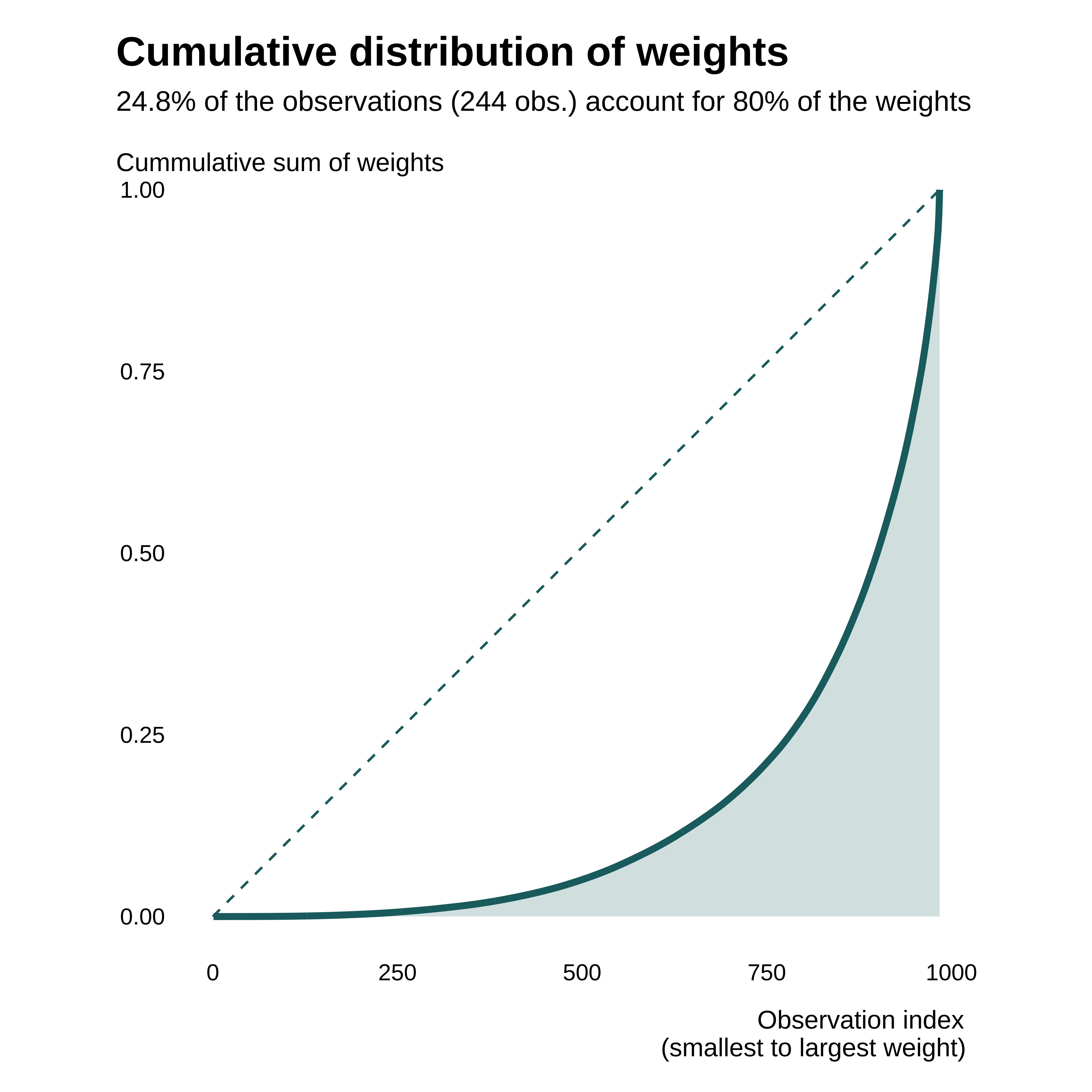

The distribution is relatively heterogeneous, some observations contributing more than others. As underlined in the subtitle, less than 25% of observations account for 80 of the weights.

We now want to identify which observations drive the identification and thus plot observation level weights:

idid_viz_weights(reg_ex, "l_gdpPercap", year, country, colors = vect_coty) +
  facet_grid(continent ~ ., scales = "free_y", space = "free_y") +
  theme(strip.text.y = element_text(angle = 0)) +
  labs(x = NULL, y = NULL)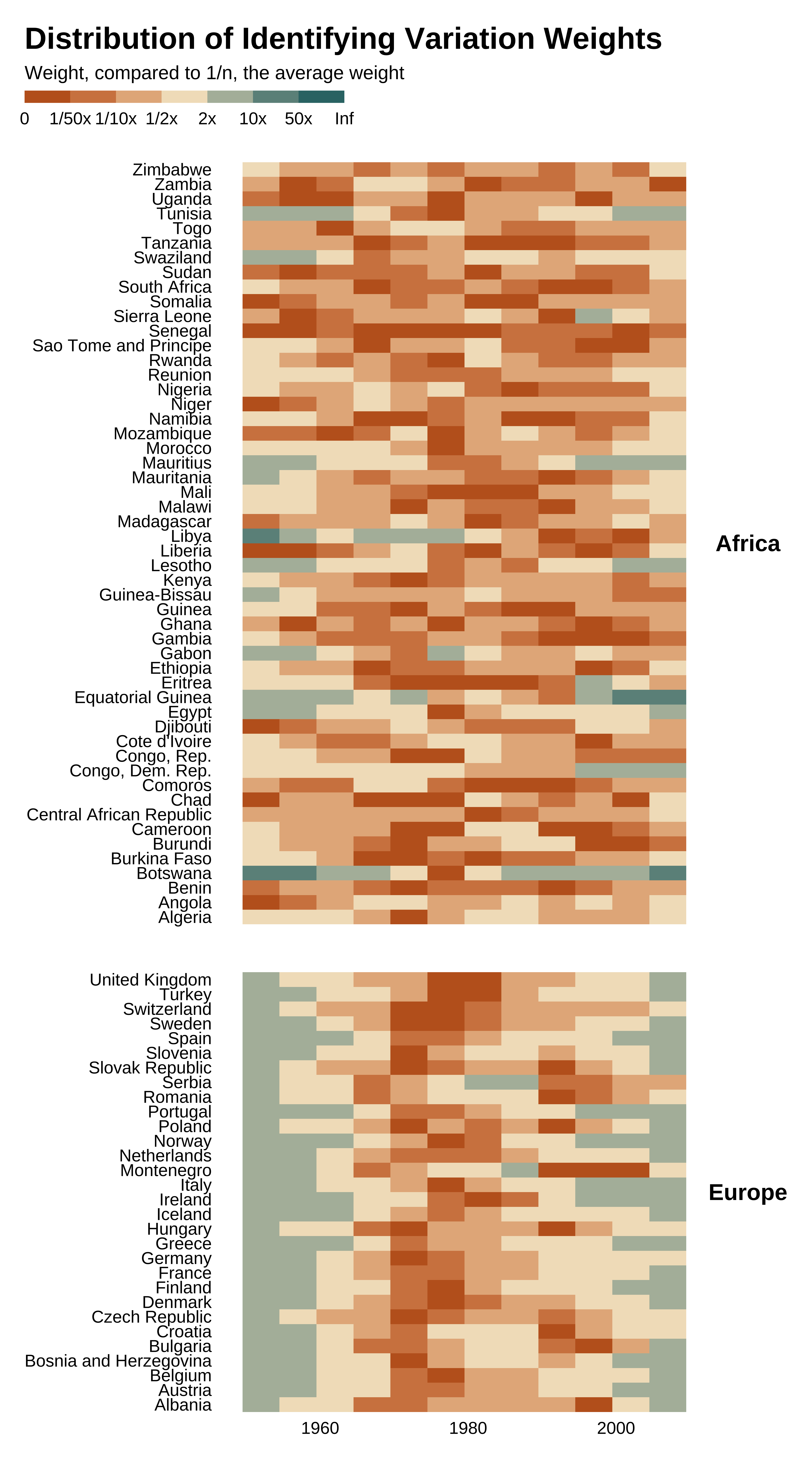 

Many observations contribute very little to identification. In particular, the distribution of weights is particularly heterogeneous: many observations contribute little to identification. In particular, observations from the middle of the period in Europe contribute little while observations in earlier and later years contribute more.

idid_viz_weights(reg_ex, "l_gdpPercap", decade, continent, colors = vect_coty) +
  facet_grid(continent ~ ., scales = "free_y", space = "free_y") +
  theme(strip.text.y = element_text(angle = 0)) +
  labs(x = NULL, y = NULL)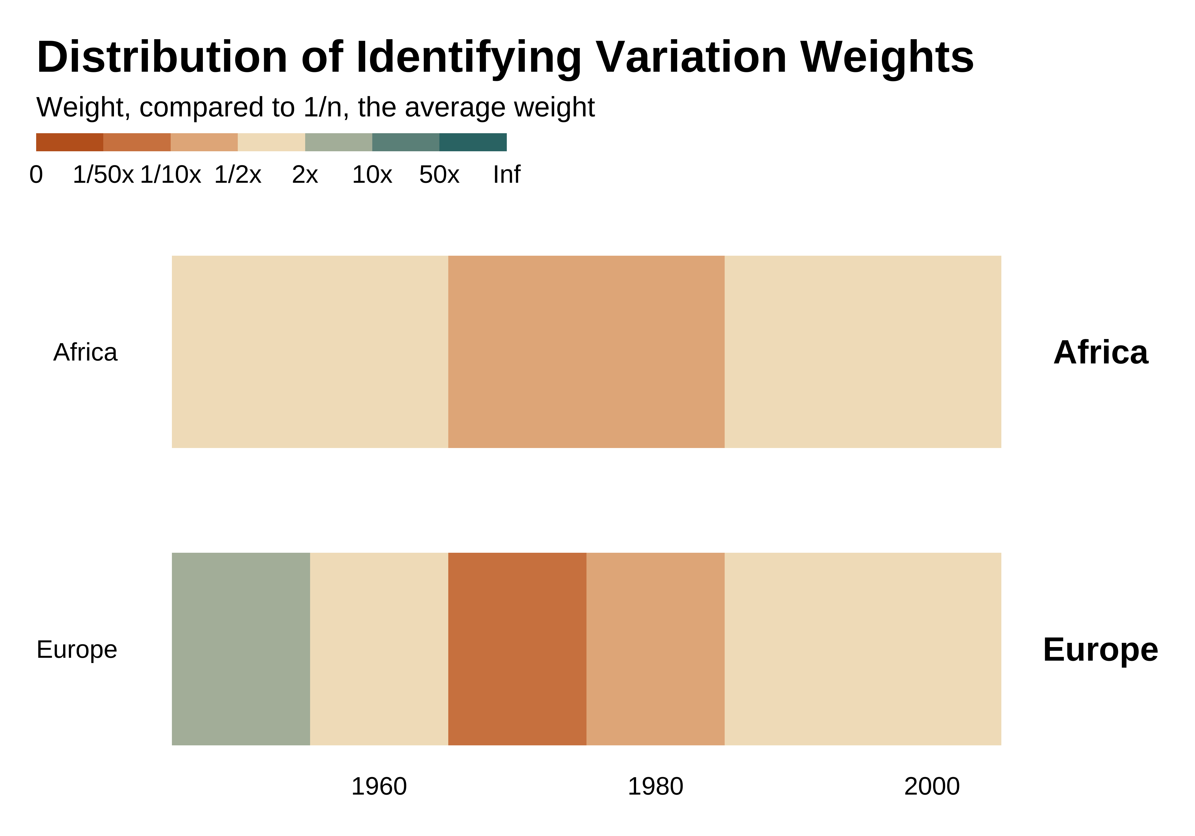

idid_viz_weights(reg_ex, "l_gdpPercap", var_x = decade, colors = vect_coty) +
  labs(x = NULL)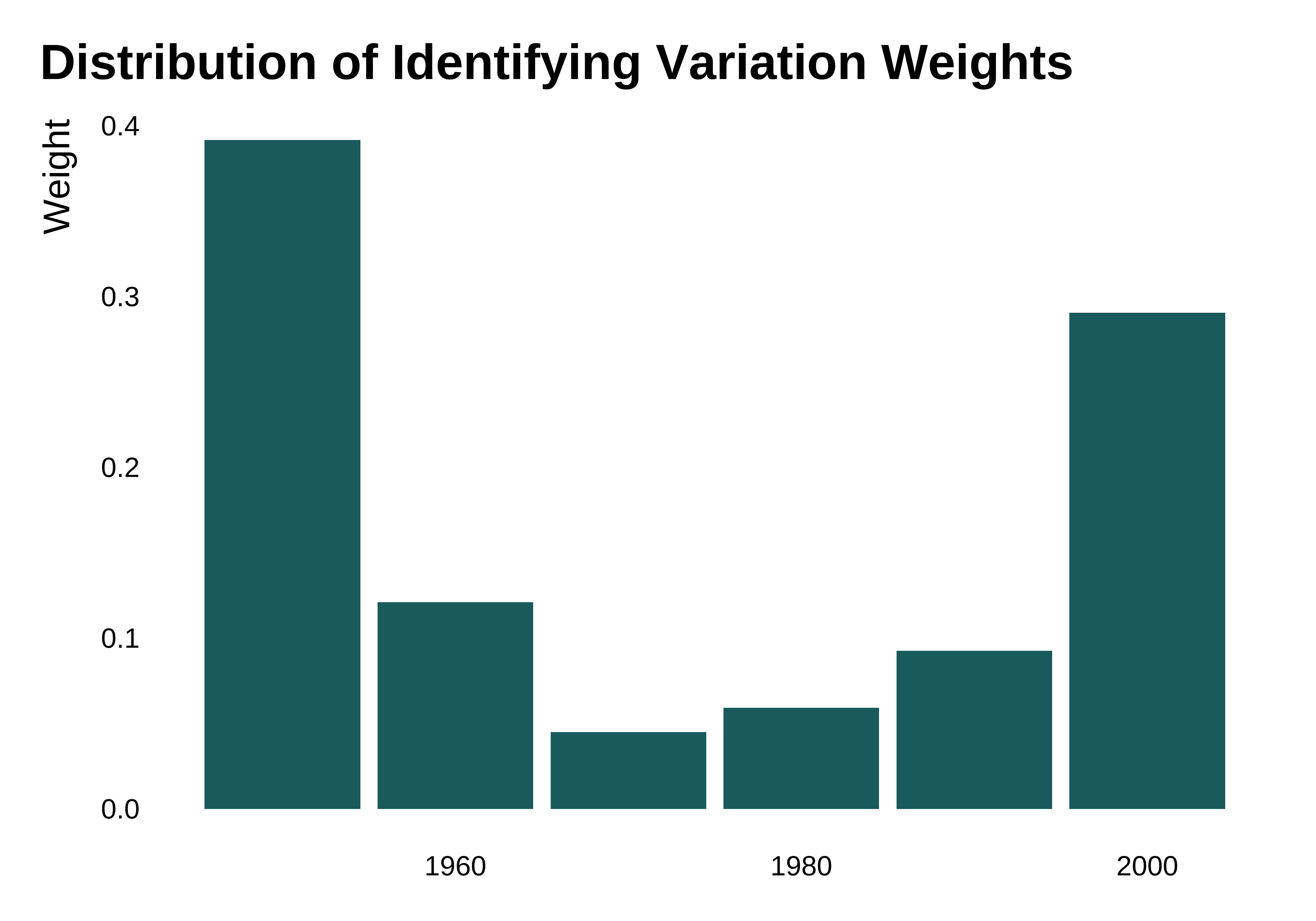 

A map may also help visualization in some cases. Here it is less useful as the variation comes mostly from years, a feature confirmed by identifying the variable that yields the most heterogeneous between-groups differences in weights (i.e. the largest between-groups variance).

idid_grouping_var(
  reg_ex, 
  "l_gdpPercap", 
  grouping_vars = c("country", "continent", "year")
) |> 
  as_tibble() |> 
  knitr::kable(col.names = c("Grouping Variable", "Variance of Weights Across Groups"))

Grouping Variable	Variance of Weights Across Groups
year	0.0052400
continent	0.0005855
country	0.0001945

world_sf <- rnaturalearth::ne_countries(scale = "medium", returnclass = "sf") |> 
  mutate(iso_alpha = adm0_a3)

#define a projection
proj_globe <-
  coord_sf(crs = "+proj=ortho +lon_0=30 +lat_0=28", expand = FALSE) 

idid_viz_weights_map(
  reg_ex, "l_gdpPercap", world_sf, "iso_alpha", colors = vect_coty) +
  proj_globe +
  theme(panel.grid.major = element_line(colour = "gray90"))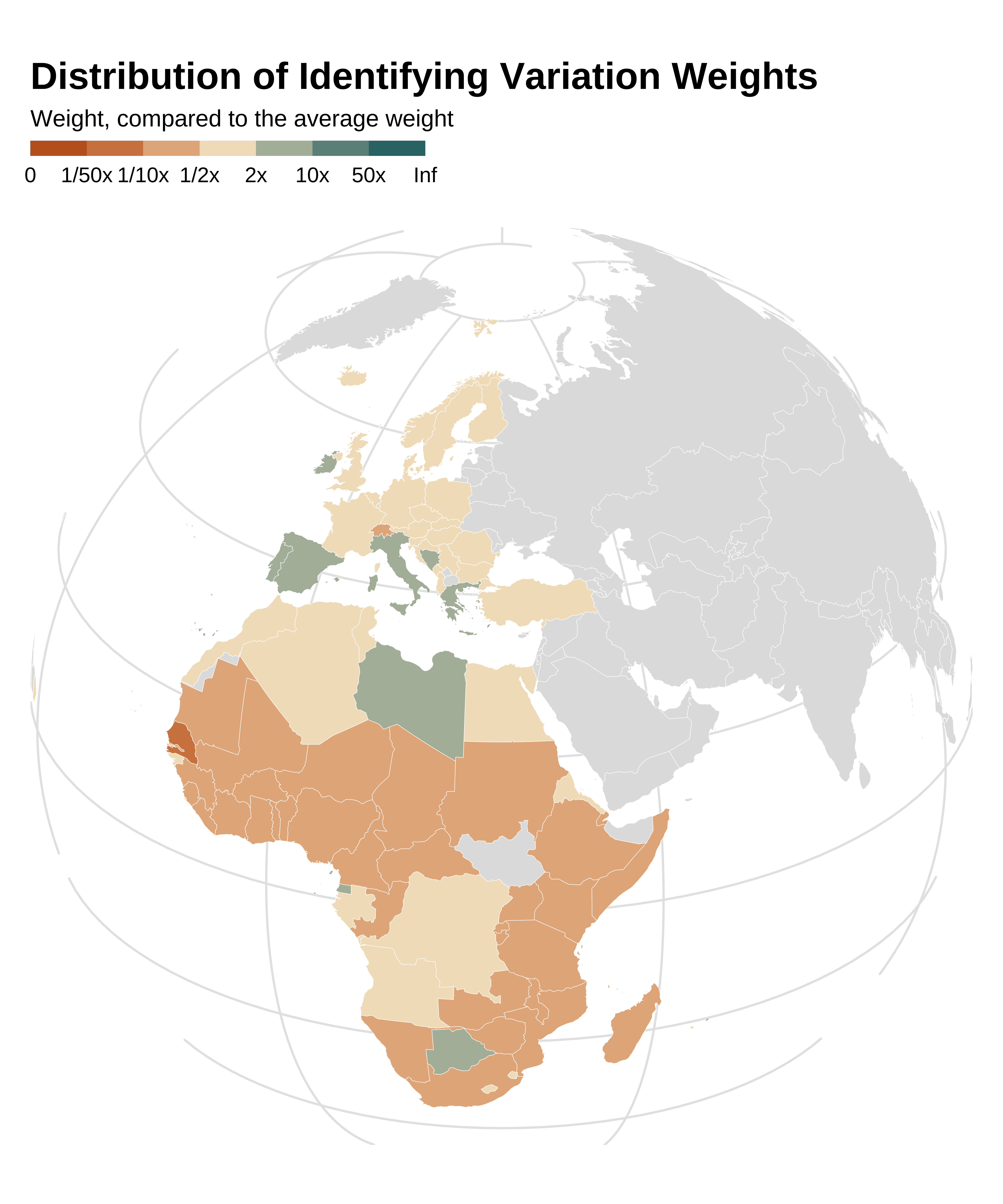 

Contributing observations

I then introduce a new metric, the number of observations that can be dropped without changing the point estimate and standard error by more than a given percentage. This procedure follows typical procedures from the influence functions literature. Concretely, the idid_viz_drop_change runs repeated estimation on subsamples of the dataset, for which various numbers of lower-weight observations have been dropped.

idid_viz_drop_change(reg_ex, "l_gdpPercap", color = col_coty)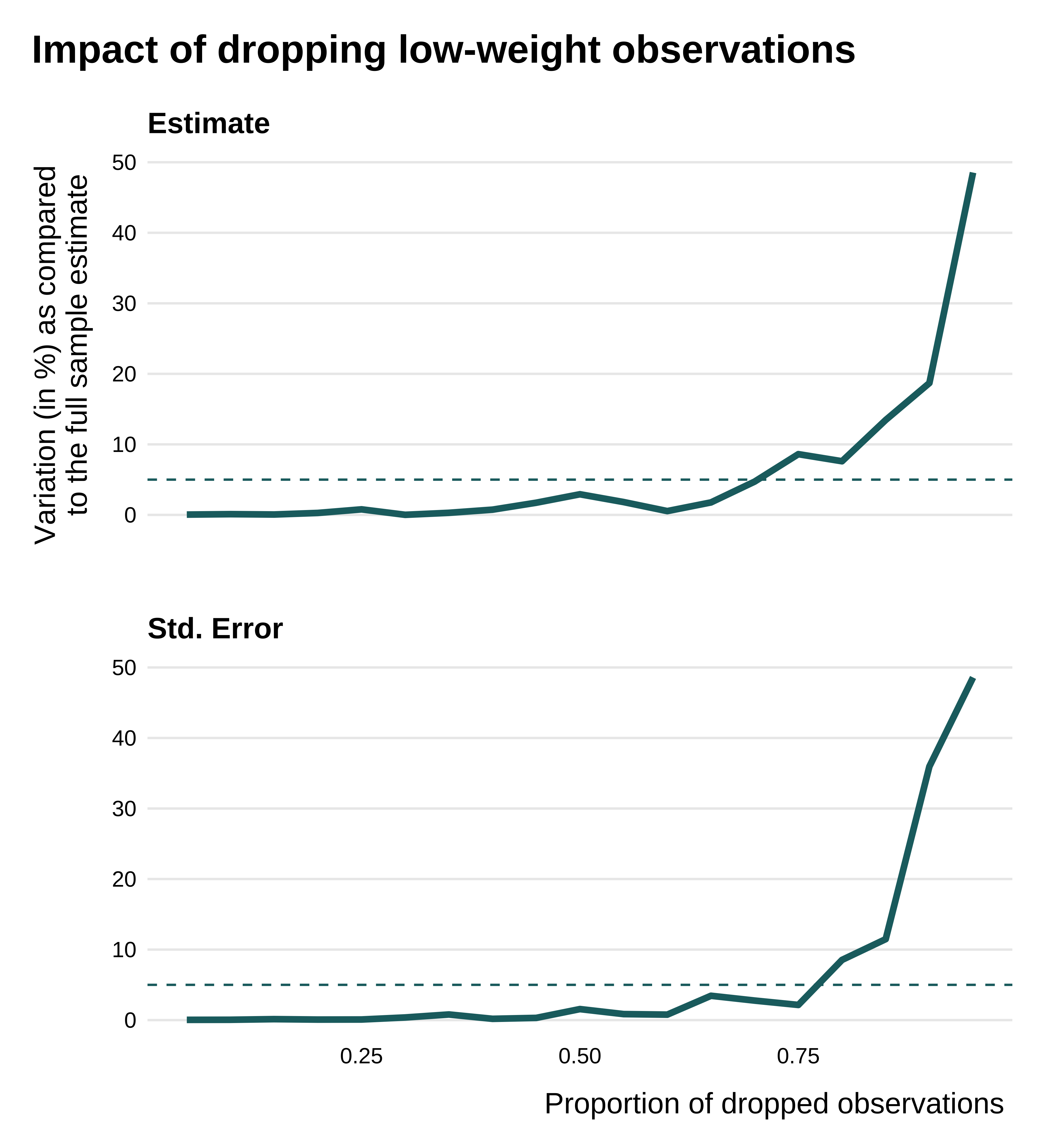

This graph highlights that considering a sample that is 70% percent smaller than the nominal sample would not change the results by more than 5%¹:

idid_drop_change(reg_ex, "l_gdpPercap", prop_drop = 0.70) |>
  kable(
    col.names = c(
      "Proportion of dropped observations",
      "Proportion of change in pt est.",
      "Proportion of change in se."
    )
  )

Proportion of dropped observations	Proportion of change in pt est.	Proportion of change in se.
0.7	0.0472294	-0.0276941

Here are the output of each regression:

modelsummary(reg_ex, gof_omit = "AIC|BIC|R2 Within")

l_gdpPercap	8.041
	(0.860)
Num.Obs.	984
R2	0.881
R2 Adj.	0.870
RMSE	4.72
Std.Errors	by: country
FE: country	X

The effective sample is defined as the set of observations that remains after dropping low-weight observations up to affecting the estimate by 5% (point estimate or s.e.):

col_names_contrib_stats <- c(
  "Initial sample size",
  "Nominal sample size",
  "Effective sample size",
  "Proportion of obs. in the effective sample"
)

idid_contrib_stats(reg_ex, "l_gdpPercap") |>
  kable(col.names = col_names_contrib_stats)

Initial sample size	Nominal sample size	Effective sample size	Proportion of obs. in the effective sample
984	984	246	0.25

Here, the effective sample size is 4 times smaller than the nominal sample size.

Based on that, we can characterize the effective sample:

idid_viz_contrib(reg_ex, "l_gdpPercap", decade, country, colors = vect_coty) +
  facet_grid(continent ~ ., scales = "free_y", space = "free_y") +
  theme(strip.text.y = element_text(angle = 0)) +
  labs(x = NULL, y = NULL)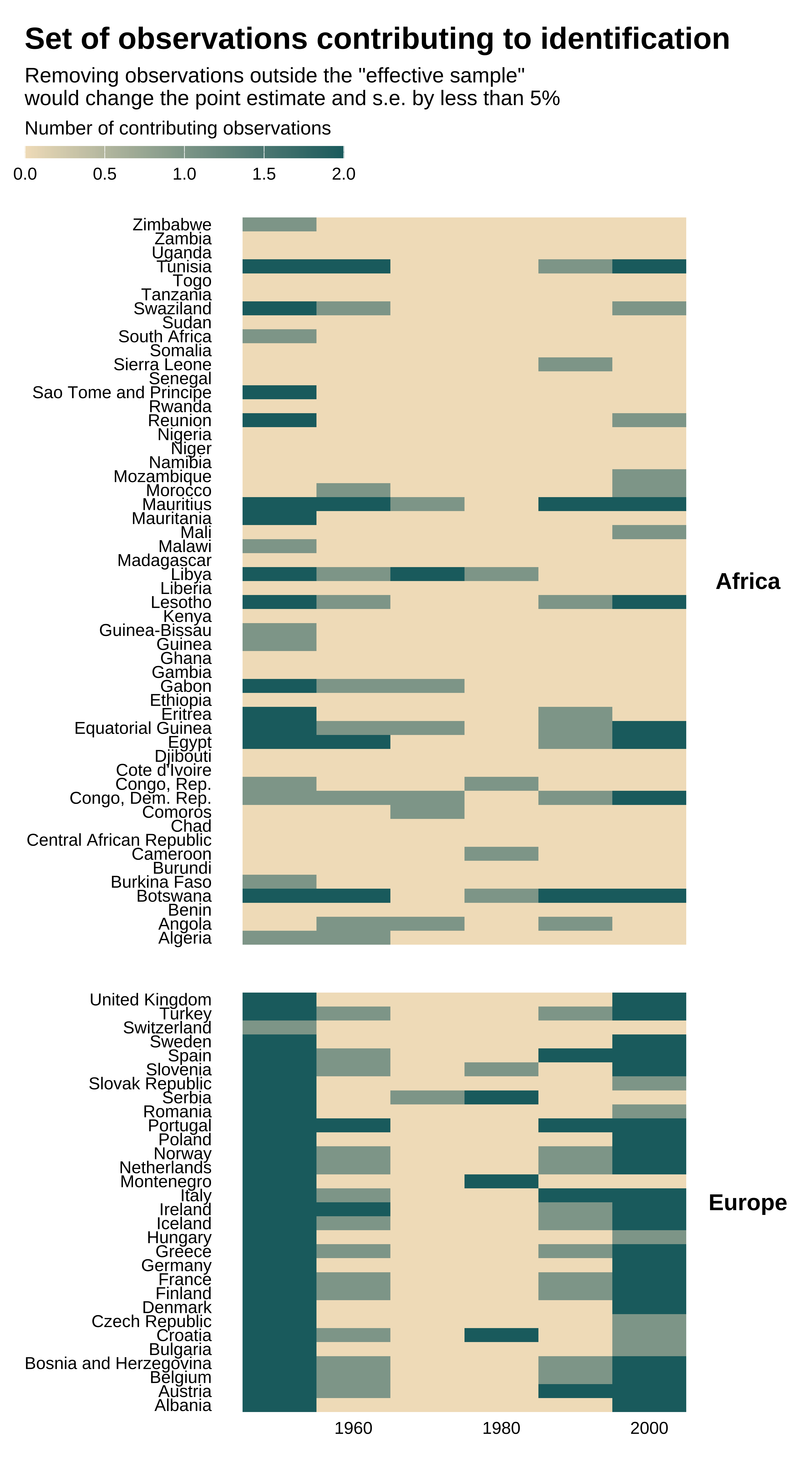 

idid_viz_contrib(reg_ex, "l_gdpPercap", decade, order = "y", colors = vect_coty) +
  facet_grid(continent ~ ., scales = "free_y", space = "free_y") +
  theme(strip.text.y = element_text(angle = 0)) +
  labs(x = NULL)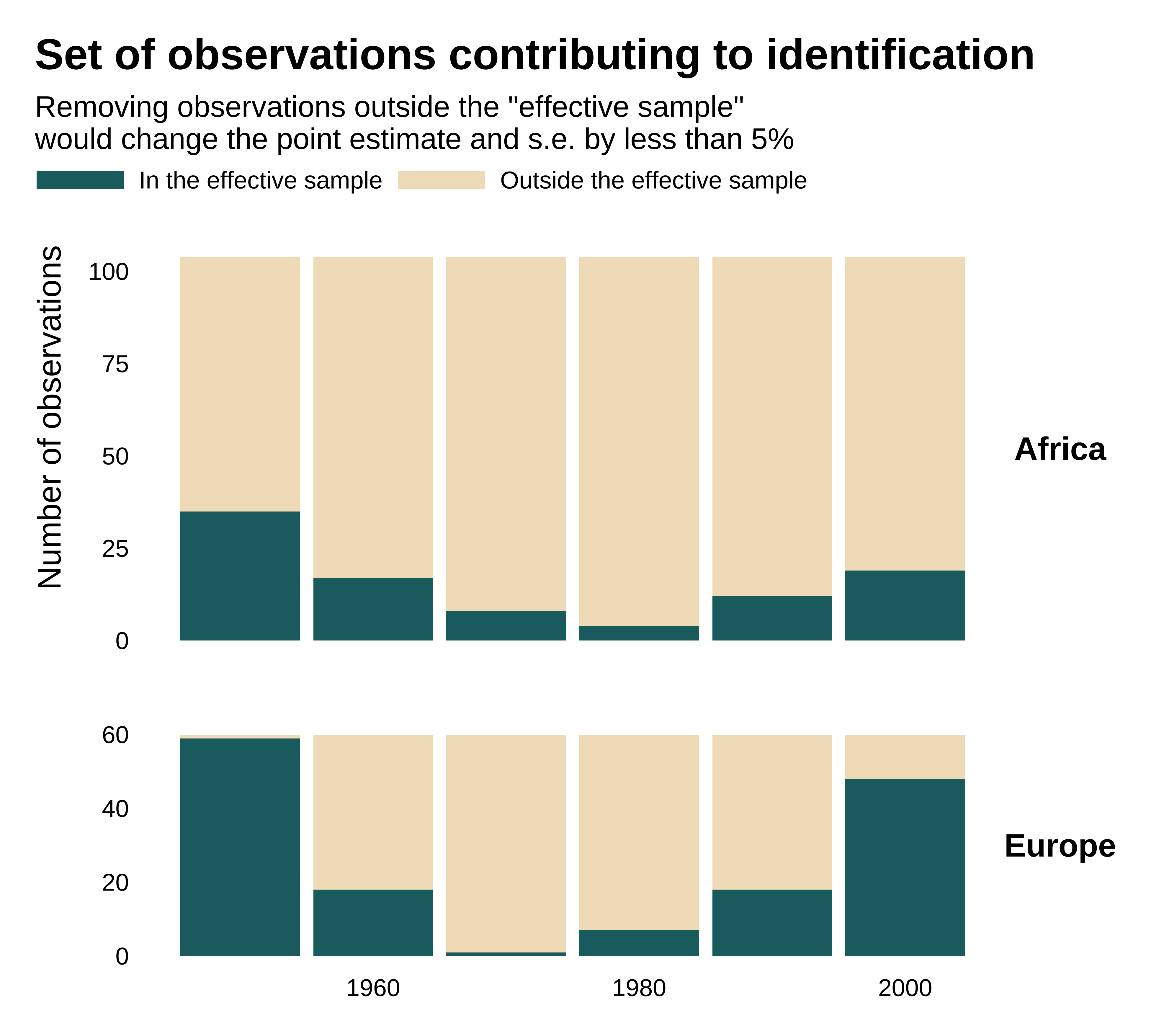 

idid_viz_contrib_map(reg_ex, "l_gdpPercap", world_sf, "iso_alpha", colors = vect_coty) +
  proj_globe +
  theme(panel.grid.major = element_line(colour = "gray90"))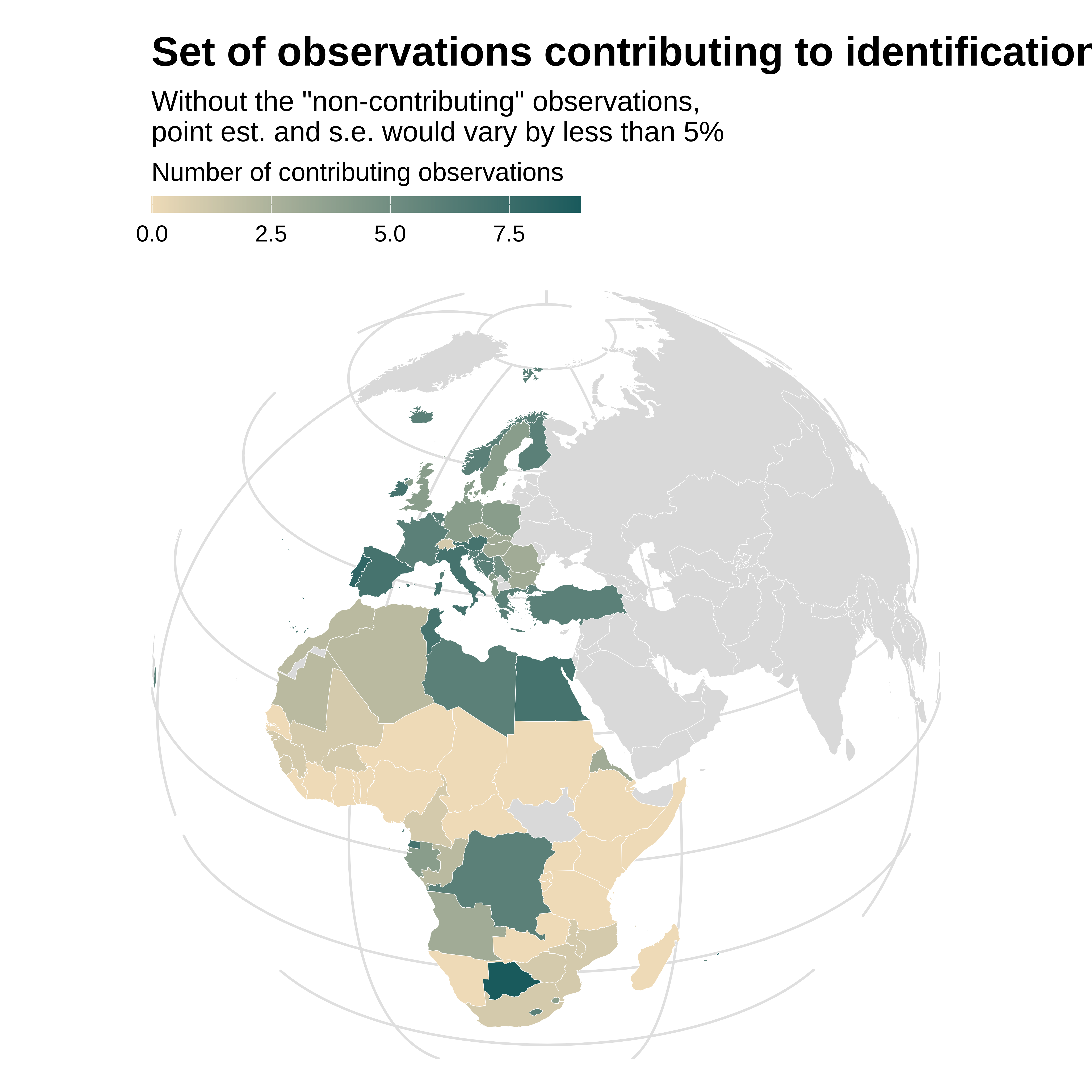 

A large number of observations from Africa and from the middle of the period do not actually contribute to identification. The effective sample is not representative of the whole set of countries and observations.

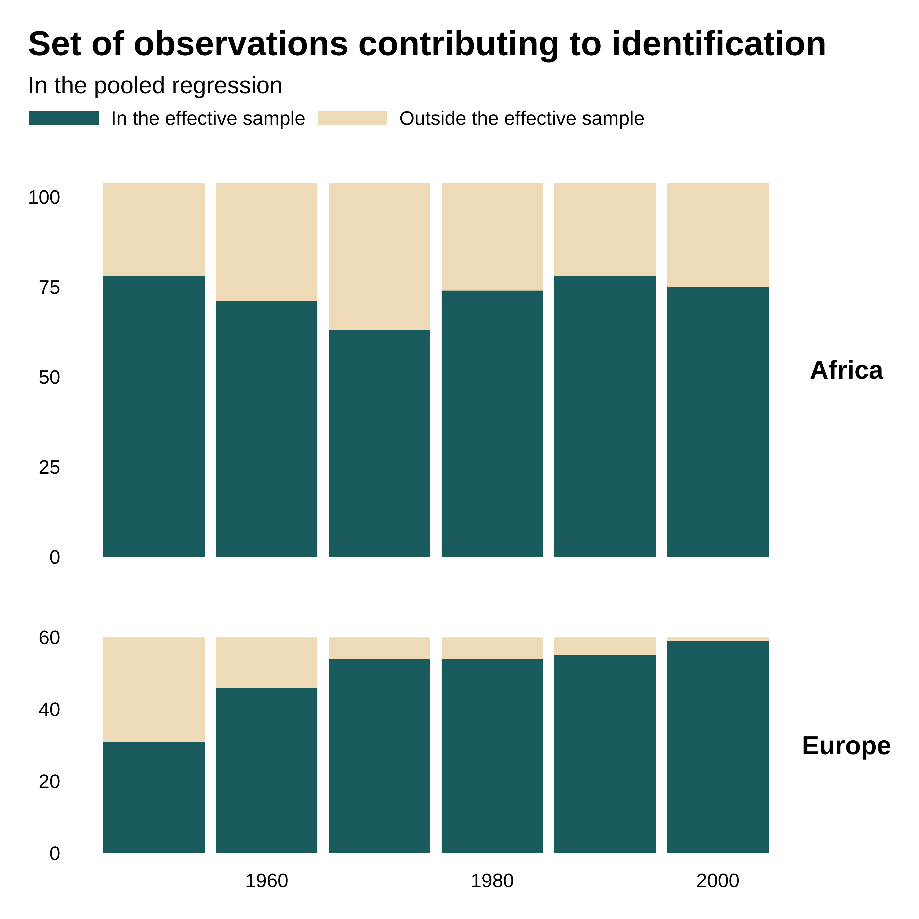
Comparison to the pooled regression

As compared, in the pooled regression, ie without fixed effects, the contributing observations are more evely distributed and the effective sample larger:

Show code

reg_pooled <- feols(gapminder_sample, lifeExp ~ l_gdpPercap, cluster = "country")

idid_viz_contrib(reg_pooled, "l_gdpPercap", decade, colors = vect_coty) +
  facet_grid(continent ~ ., scales = "free_y", space = "free_y") +
  theme(strip.text.y = element_text(angle = 0)) +
  labs(
    x = NULL, 
    y = NULL, 
    subtitle = "In the pooled regression"
  ) 

Show code

idid_viz_contrib_map(reg_pooled, "l_gdpPercap", world_sf, "iso_alpha", colors = vect_coty) +
  proj_globe +
  theme(panel.grid.major = element_line(colour = "gray90")) +
  labs(subtitle = "In the pooled regression")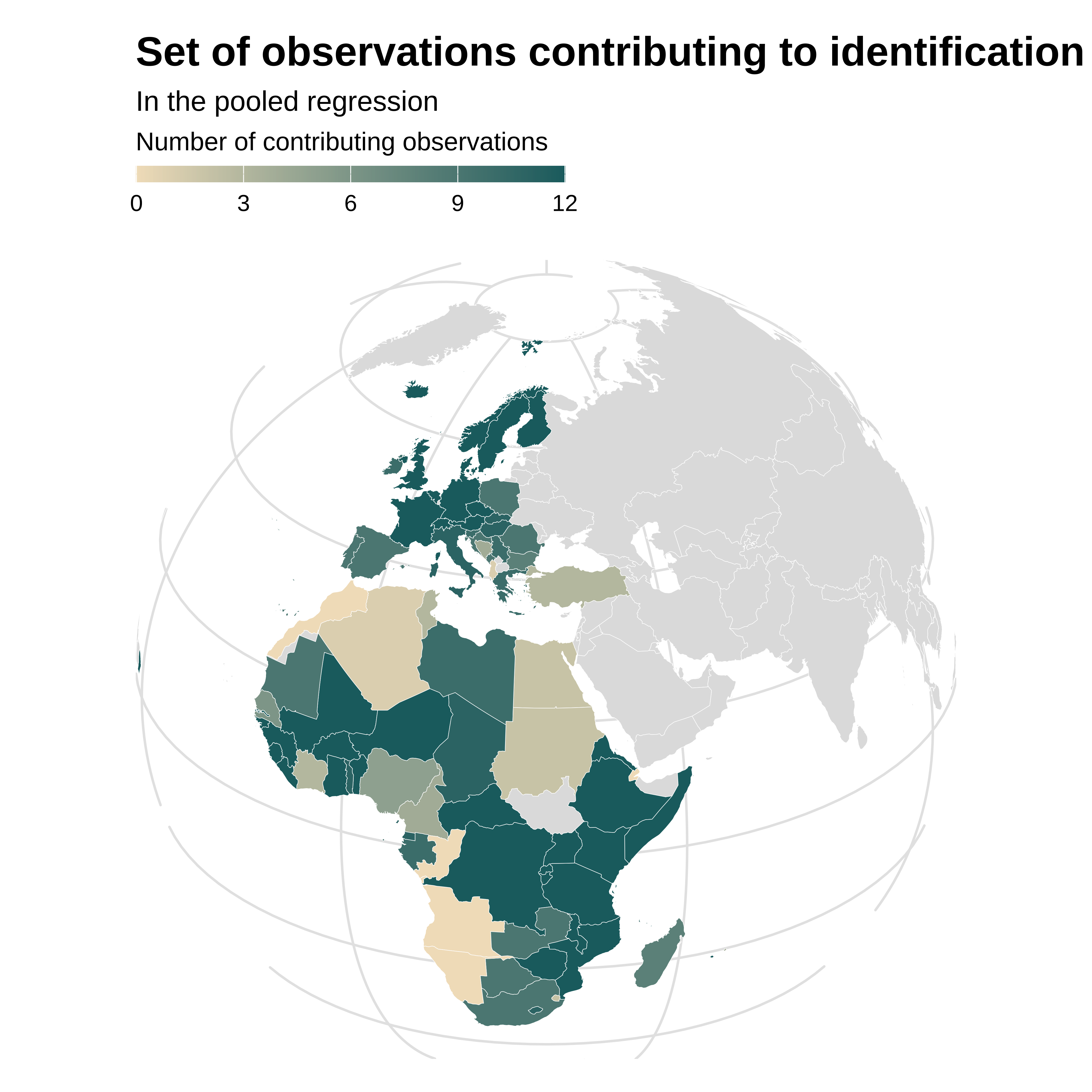

The effective sample is much larger:

map(list(reg_ex, reg_pooled), idid_contrib_stats, var_interest  = "l_gdpPercap") |>
  list_rbind() |>
  kable(col.names = col_names_contrib_stats)

Initial sample size	Nominal sample size	Effective sample size	Proportion of obs. in the effective sample
984	984	246	0.25
984	984	738	0.75

The fixed-effects change the estimand but also affect the effective sample and its size.

---

1. This 5% threshold is completely arbitrary and other values could and should be considered↩︎