Visualization of Identifying Variation Weights — idid_viz

Makes a graph to visualize the identifying variation weights (a heatmap or a bar chart, depending on the number of dimensions specified)

Usage

idid_viz_weights(
  reg,
  var_interest,
  var_x,
  var_y,
  order = "",
  colors = c("#C25807", "#FBE2C5", "#300D49"),
  keep_labels = TRUE,
  ...
)

Arguments

reg: A regression object.
var_interest: A string. The name of the main variable of interest.
var_x: A variable in the data set used in reg to plot on the x-axis.
var_y: A variable in the data set used in reg to plot on the y-axis (optional). If not specified, produces a bar chart.
order: A string (either "x", "y" or "xy") describing whether the graph should be order, along the x or y axis or both. If anything else is specified, no specific ordering will be applied.
colors: A string vector of colors for the palette. I recommend to pass a vector of 3 distinct colors, with a lighter color in the middle, constituting a diverging scale. It allows a clear distinction between contributing and non contributing observations.
keep_labels: A boolean (optional). If FALSE, removes y labels and ticks. This option is useful for panels with a large number of individuals.
...: Additional elements to pass to the regression function when partialling out controls.

Value

A ggplot2 graph of identifying variation weights.

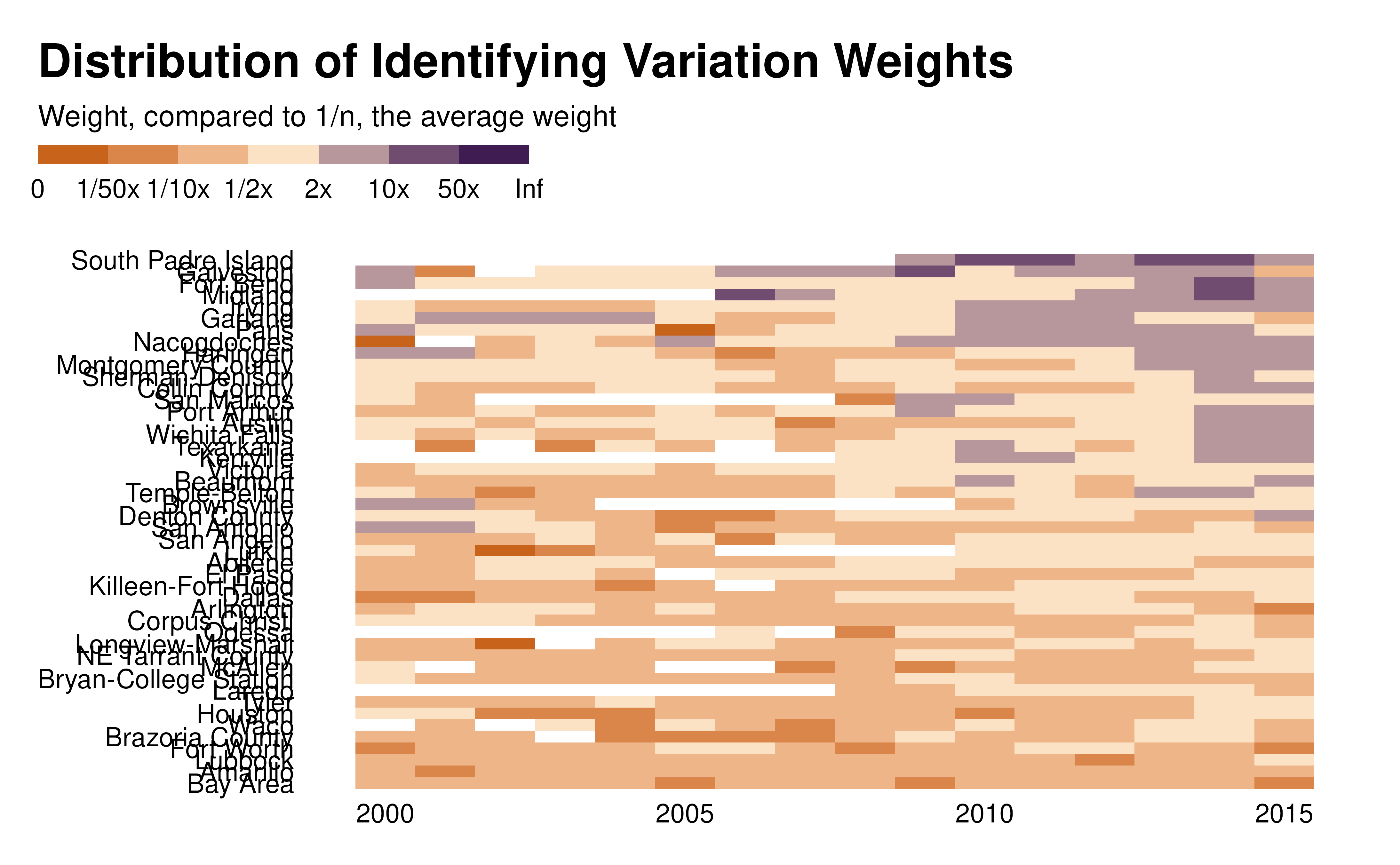
If var_y is specified, returns a heatmap whose color represents a categorized version of the identifying variation weights (the categorization prevents the vizualisation from being driven by extremely large weights).

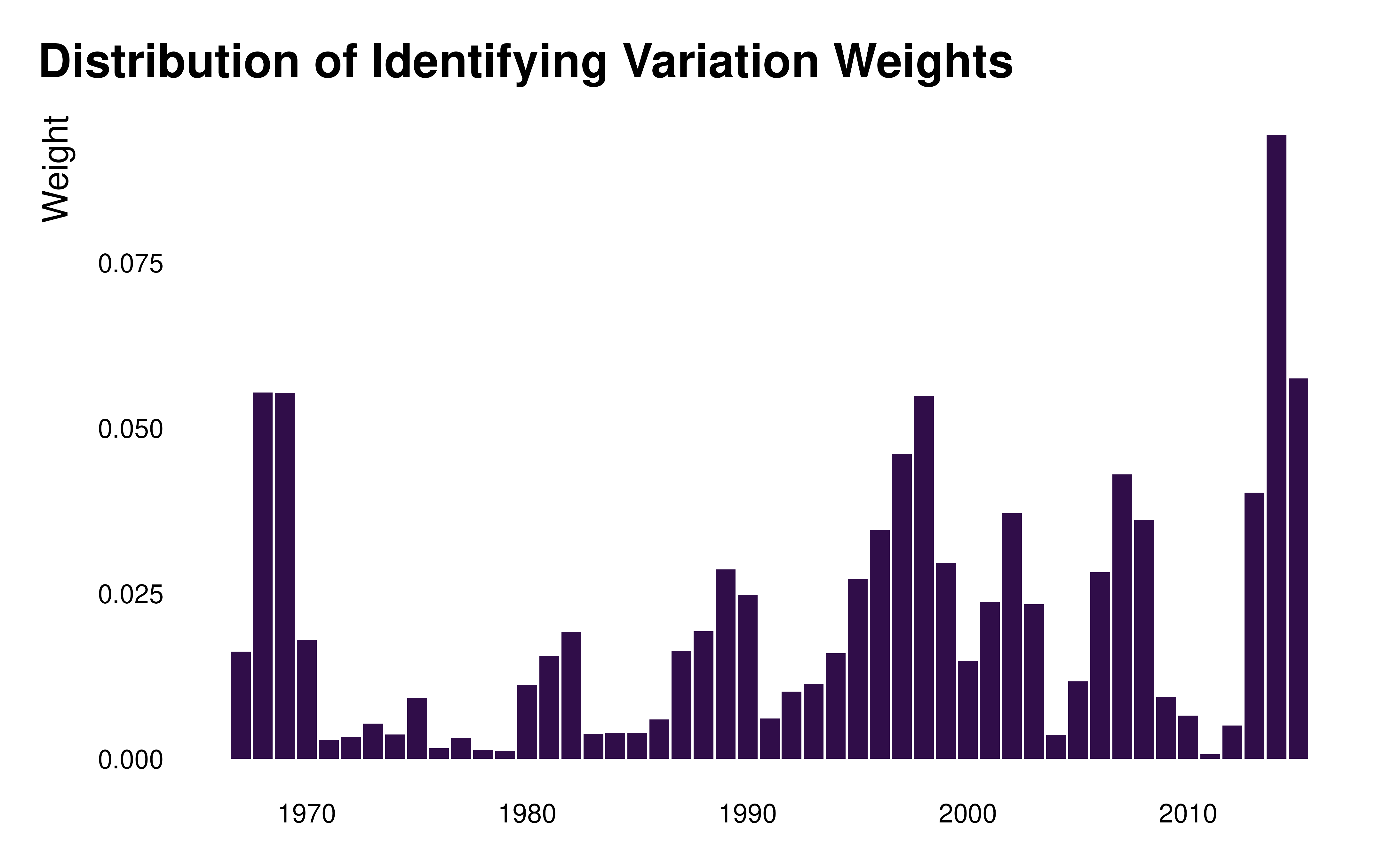
If var_y is not specified, returns a bar chart representing the weights in each group.

Details

If there is more than on observation by group (i.e. for one category in var_x or in var_x x var_y), the weight of the group is computed by summing individual weights in that group, removing missing values.

Examples

# example one dimension
reg_ex_one_dim <- ggplot2::economics |>
  transform(year = substr(date, 1, 4) |> as.numeric()) |>
  lm(formula = unemploy ~ pce + uempmed + psavert + pop + year)

idid_viz_weights(reg_ex_one_dim, "pce", var_x = year) +
  ggplot2::labs(x = NULL)


# example with two dimensions
reg_ex_two_dim <- ggplot2::txhousing |>
  lm(formula = log(sales) ~ median + listings + as.factor(date) + city)

idid_viz_weights(reg_ex_two_dim, "median", year, city, order = "y") +
  ggplot2::labs(x = NULL, y = NULL)
#> Warning: Removed 1434 rows containing non-finite outside the scale range
#> (`stat_log_weight()`).