Show the packages used in this document
library(tidyverse)
library(knitr)
library(mediocrethemes)
library(here)
library(retrodesign)
library(haven)
library(janitor)
# library(DT)
# library(kableExtra)

set_mediocre_all(pal = "coty")
Motivation and assumptions
Despite being very broad, the analysis of studies published in top economics journals I implement here relies on assumptions regarding the effect size that may lack theoretical grounding and that may seem arbitrary, to some extent. To overcome this limitation and to be able to make more grounded hypotheses for true effect sizes, I focus on studies using IVs. They allow to compare the OLS estimate to the 2SLS, to evaluate whether the IV would have enough power to “detect” the OLS estimate and to compute exaggeration of the IV if the true effect was close to the OLS point estimate.
In this document, I therefore leverage the reviews by Young (2022) and Lal et al. (2024) to explore potential exaggeration of the IVs in the economics and political science literature.
Here too, I am not claiming that the OLS is the true effect. I am however evaluating the ability of the IV to retrieve an effect of the magnitude of the OLS. It may seem reasonable to expect the design of the IV to be good enough to accurately capture this effect, if it was the true effect.
To compute these analyses, I use the standard errors reported by the authors of each analysis, even though some of these are likely understated, as underlined by Young (2022) and Lal et al. (2024). This approach is therefore conservative.
IVs in the Economics Literature
I first compute the aforementioned measures for the economics literature, leveraging data gathered in Young (2022). This paper analyzes 30 papers published in journals of the American Economics Association published through July 2016, for a total of 1309 2SLS regressions. To carry out his analysis, Young retrieved all these estimates and associated standard errors.
This analysis yielded several findings, including some that are of particular interest for the present paper:
- When errors are non-iid, first stage F-statistics are often uninformative when the strength of the first stage weakens and in high-leverage settings
- Conventional t-tests regularly overstate precision
- 2SLS confidence intervals are large and almost always include OLS point estimates
- 2SLS estimates are often substantially larger than their OLS counterpart
Data
To do so, I first use data from the paper’s replication package. These data can be downloaded here. The file of interest (Base.dta) is stored in the results folder. For each of the 1309 estimates, it contains the IV and OLS point estimates as well as whether the result is a headline result or not. I import it.
Show code
point_estimates_young <- read_dta(
  here("inputs", "young", "Base.dta")
  ) |>
  janitor::clean_names() |>
  select(reg_num, paper, headline, estimate_iv = biv, estimate_ols = bols) |>
  mutate(headline = as.logical(headline)) |>
  mutate(ratio_iv_ols = abs(estimate_iv/estimate_ols))
To implement power calculations, I also need associated standard errors. However, these data are not publicly available, to avoid offering the possibility of pinpointing a particular study. Alwyn Young very kindly shared part of his data with me, allowing me to run these analyses. He provided me with both the ratio of the IV and OLS point estimates over the standard error of the IV estimator. This prevents the identification of the paper from their point estimates and associated standard errors but still allows me to compute the measures of interests. This data transformation can be seen as some sort of normalization. I import this data.
IV/OLS ratios
First, I compute the ratio of the 2SLS estimates over the corresponding OLS estimates in order to further explore the difference in magnitude between the two estimates. Young already underlined that “the absolute difference of the 2SLS and OLS point estimates is greater than 0.5 times the absolute value of the OLS point estimate in .73 of headline regressions and greater than 5.0 times that value in .24 of headline regressions”. I implement a similar analysis to homogenize it with my analysis of estimates of short-term health effects of air pollution. I compute the ratios of the two 2SLS estimates over the corresponding OLS:
Show code
point_estimates_young |>
  group_by(headline) |>
  summarise(
    median_ratio = median(ratio_iv_ols),
    third_quartile = quantile(ratio_iv_ols, 0.75)
  ) |>
  round(2) |>
  mutate(headline = ifelse(headline, "Yes", "No")) |>
  kable(
    col.names = c("Headline result",
                  "Median 2SLS/OLS ratio",
                  "3rd quartile 2SLS/OLS ratio")
)| Headline result | Median 2SLS/OLS ratio | 3rd quartile 2SLS/OLS ratio |
|---|---|---|
| No | 2.44 | 5.49 |
| Yes | 2.26 | 5.36 |
The distribution for headline results highlights important heterogeneity (sd of the ratios 210.6310918).
Show code
point_estimates_young |>
  filter(headline == 1) |>
  ggplot() +
  geom_segment(
    aes(x = ratio_iv_ols, xend = ratio_iv_ols, y = 0, yend = 1),
    linewidth = 0.8,
    alpha = 0.5
  ) +
  geom_vline(
    aes(xintercept = median(ratio_iv_ols)),
    linewidth = 1,
    linetype = "solid"
  ) +
  scale_x_log10() +
  labs(
    title = "Some 2SLS headline estimates are much larger than the OLS",
    x = "Ratio 2SLS/OLS",
    y = NULL,
    caption = "The black line represents the median"
  ) +
  theme(panel.grid.major.y = element_blank(), axis.text.y = element_blank()) +
  annotate(
    geom = "curve",
    x = 2.4, y = 0.8, xend = 4.5, yend = 1.05,
    curvature = .5,
    color = "black",
    linewidth = 0.6,
    arrow = arrow(length = unit(2, "mm"), type = "closed")
  ) +
  annotate(
    geom = "text",
    x = 4, y = 1.15,
    label = "Median",
    hjust = "left",
    color = "black",
    size = 4,
    family = "Lato"
  )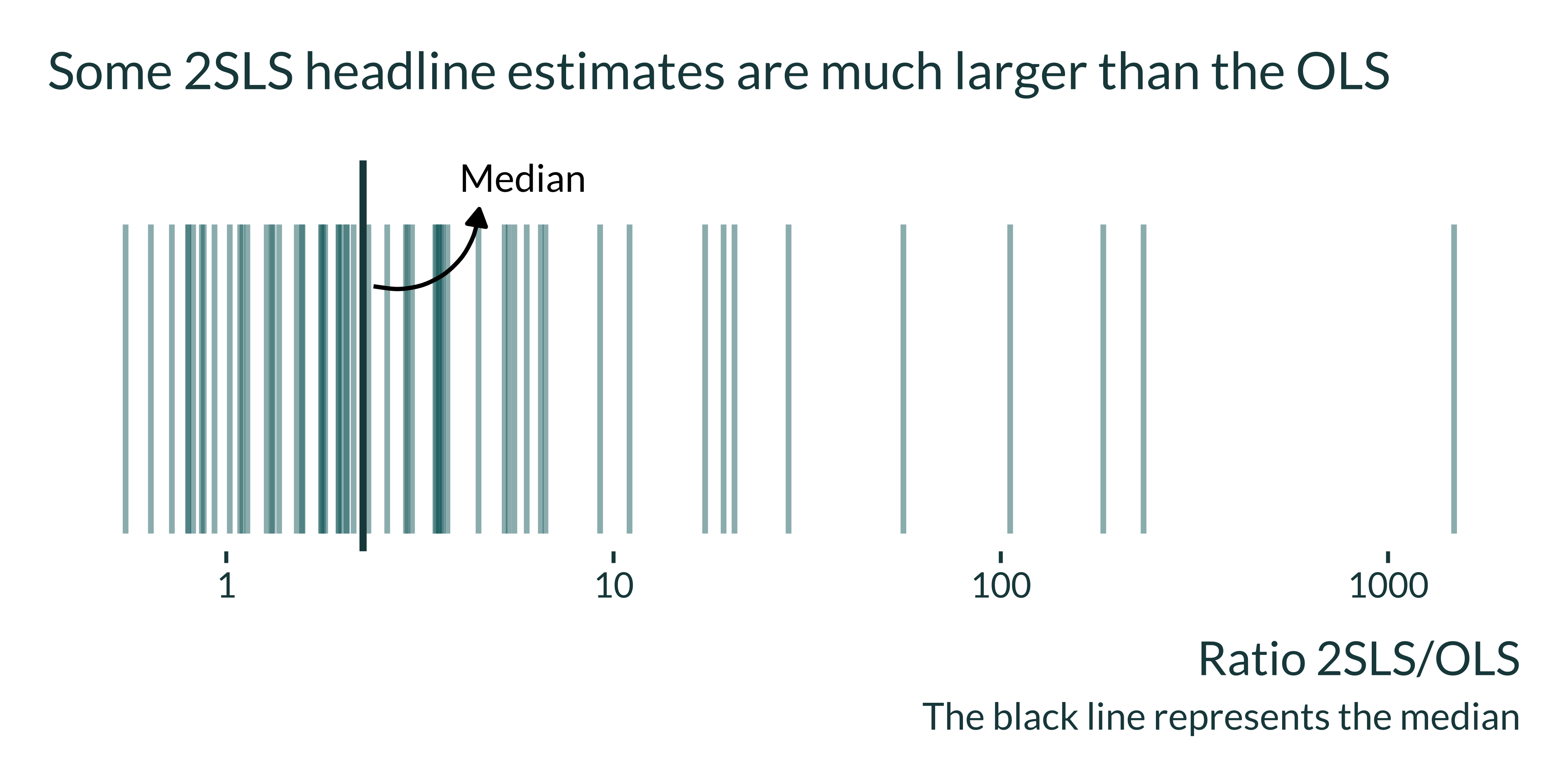
Some 2SLS point estimates are substantially larger than the corresponding OLS. Others are close or smaller but overall, most 2SLS point estimates are larger than their OLS counterpart. For all results (headline or not), the pattern is similar:
Show code
point_estimates_young |>
  arrange(ratio_iv_ols) |>
  mutate(reg_id = row_number()) |>
  filter(ratio_iv_ols > 0) |>
  ggplot(aes(x = ratio_iv_ols, y = reg_id)) +
  geom_point() +
  geom_vline(xintercept = 1) +
  scale_x_log10(n.breaks = 6) +
  labs(
    title = "Distribution of the IV/OLS ratios",
    subtitle = "Most IV estimates are larger than OLS",
    x = "IV estimate/OLS estimate",
    y = "Design identifier (ordered)",
    caption = "Each dot represents one design"
  ) +
  theme(panel.grid.major.y = element_blank(), axis.text.y = element_blank())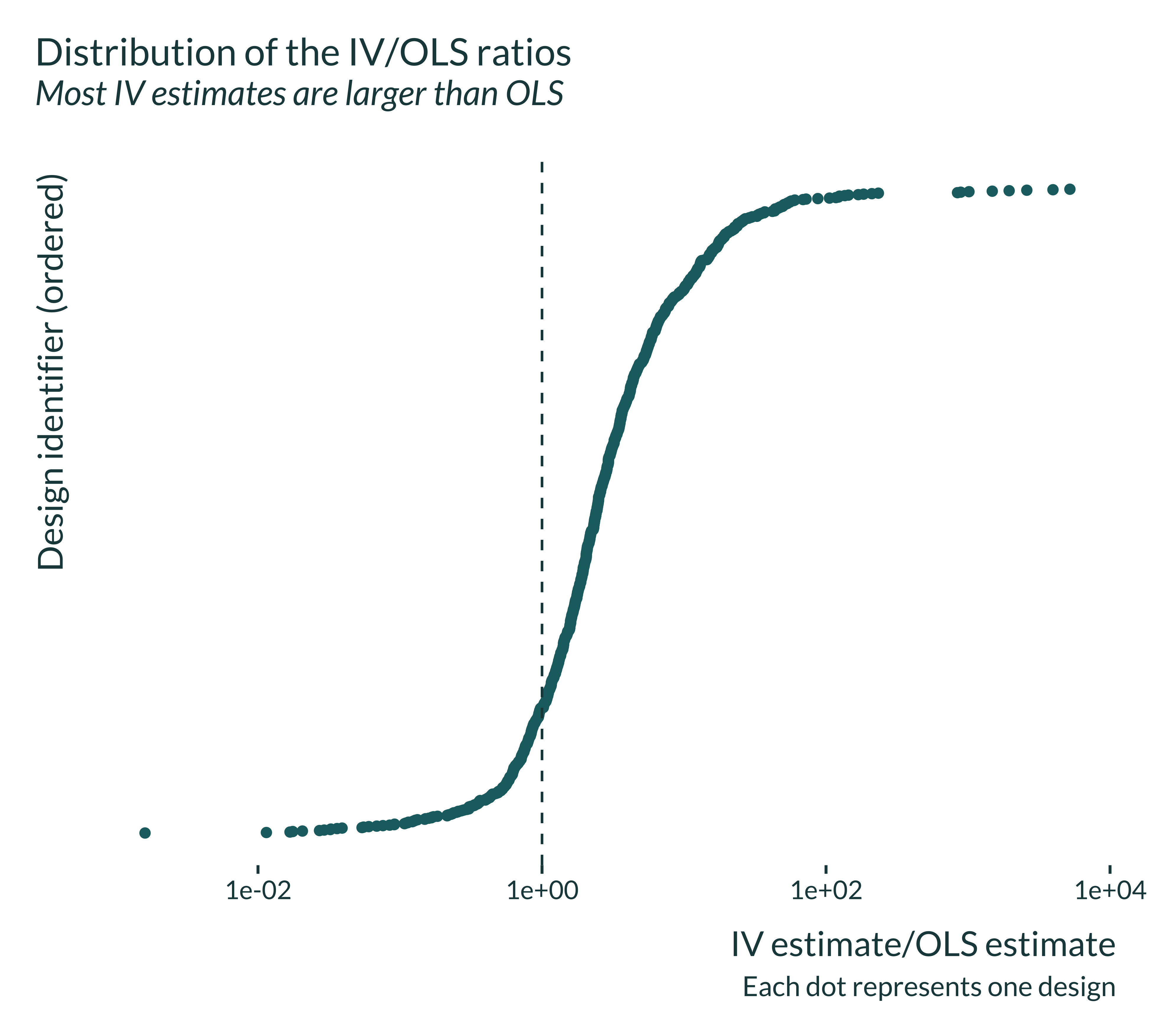
Power calculations
I then turn to the actual power calculations, computing what would be the statistical power and exaggeration if the true effect was equal to the OLS point estimate.
retro_young_ols <- snr_young |>
  mutate(
    retro = retro_design_closed_form(BolsoverSEiv, 1) |> as_tibble()
  ) |>
  unnest(retro) |>
  mutate(power = power*100)
Power
Most IV designs would not have enough power to accurately detect an effect of the magnitude of the OLS:
Show code
| Adequate Power | Number of Estimates | Proportion (%) |
|---|---|---|
| No | 1184 | 90.5 |
| Yes | 125 | 9.5 |
For significant headline results, the proportion is slightly larger:
Show code
| Adequate Power | Number of Estimates | Proportion (%) |
|---|---|---|
| No | 39 | 83 |
| Yes | 8 | 17 |
Exaggeration ratio
Many designs would display large exaggeration ratios:
Show code
retro_young_ols |>
  filter(headline) |>
  ggplot() +
  geom_segment(
    aes(x = type_m, xend = type_m, y = 0, yend = 1),
    linewidth = 0.8,
    alpha = 0.5
  ) +
  geom_vline(
    aes(xintercept = median(type_m)),
    linewidth = 1,
    linetype = "solid"
  ) +
  scale_x_log10() +
  labs(
    title = "Distribution of exaggeration ratios of IV headline designs",
    subtitle = "Many designs would display substantial exaggeration of OLS estimates",
    x = "Exaggeration ratio",
    y = NULL,
    caption = "The black line represents the median"
  ) +
  theme(panel.grid.major.y = element_blank(), axis.text.y = element_blank())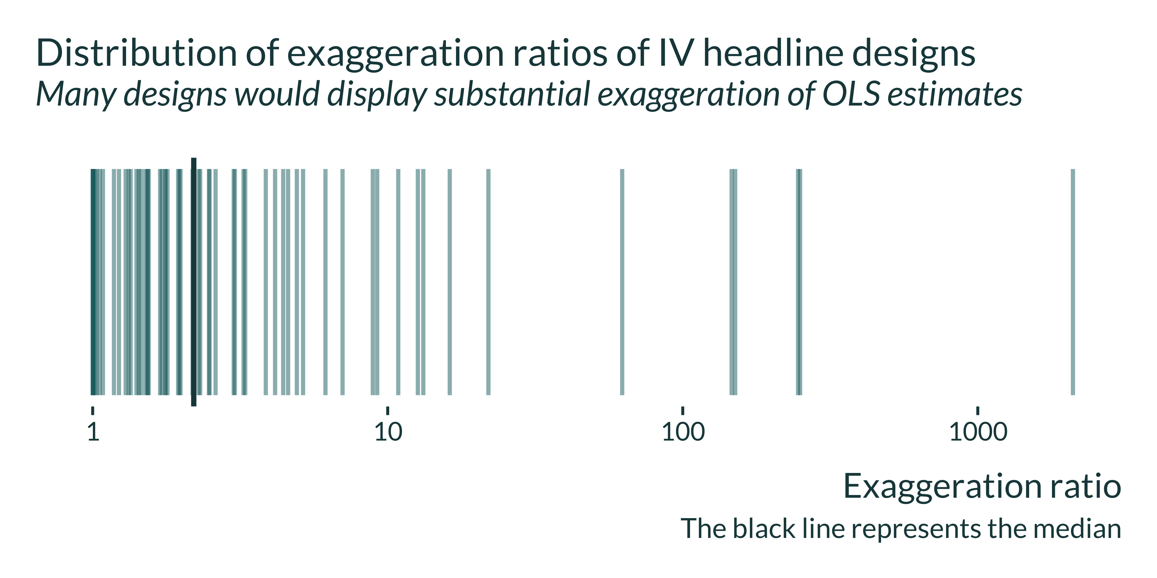
I then compute summary statistics. They reveal that exaggeration is even larger if we also consider non-headline results:
Show code
source(here("functions.R"))

retro_young_ols |>
  summary_power() |>
  mutate(results = "All", .before = 1) |>
  bind_rows(
    retro_young_ols |>
      filter(headline, signif) |>
      summary_power() |>
      mutate(results = "Significant headline", .before = 1)
  ) |>
  bind_rows(
    retro_young_ols |>
      filter(signif) |>
      summary_power() |>
      mutate(results = "All significant", .before = 1)
  ) |>
  rename_with(\(x) str_to_title(str_replace_all(x, "_", " "))) |>
kable()| Results | Median Exagg | 3rd Quartile Exagg | Prop Larger 2 | Median Power | 3rd Quartile Power |
|---|---|---|---|---|---|
| All | 3.2 | 7.7 | 72.0 | 11.8 | 28.8 |
| Significant headline | 2.0 | 3.6 | 46.8 | 25.5 | 52.5 |
| All significant | 2.4 | 4.6 | 57.9 | 18.4 | 49.2 |
Hypithetical true effect equal to half the effect found
I then reproduce a similar analysis to the one I implemented when reviewing the RDD, IV, RCT and DID literature using data from Brodeur et al. (2020), computing exaggeration under the assumption of a true effect equal to half of the point estimate obtained.
Show code
retro_young_half <- snr_young |>
  mutate(
    retro = retro_design_closed_form(BivoverSEiv/2, 1) |> as_tibble()
  ) |>
  unnest(retro) |>
  mutate(power = power*100)

summary_power(retro_young_half) |>
  mutate(results = "all", .before = 1) |>
  bind_rows(
    retro_young_half |>
      filter(headline) |>
      summary_power() |>
      mutate(results = "headline", .before = 1)
  ) |>
  bind_rows(
    retro_young_half |>
      filter(signif) |>
      summary_power() |>
      mutate(results = "significant", .before = 1)
  ) |>
  rename_with(\(x) str_to_title(str_replace_all(x, "_", " "))) |>
kable()| Results | Median Exagg | 3rd Quartile Exagg | Prop Larger 2 | Median Power | 3rd Quartile Power |
|---|---|---|---|---|---|
| all | 2.4 | 4.2 | 64.1 | 17.6 | 32.6 |
| headline | 2.0 | 2.5 | 50.8 | 24.2 | 37.4 |
| significant | 1.8 | 2.2 | 33.8 | 30.9 | 46.4 |
Power is lower here than in the analysis of Brodeur et al’s data because here I included all estimates and did not limit the sample to statistically significant results.
IVs in the Political Science Literature
I then turn to a comparable review, Lal et al. (2024) but in political science. This paper replicates the 67 papers (70 designs) replicable papers published in three top political science journals (American Political Science Review, American Journal of Political Science, and the Journal Of Politics) between 2010 and 2022. They focus on design with one endogenous variable.
This paper also provides a set of results that are of particular interest to the present paper:
- IV in political science estimates are often very imprecise and this uncertainty is underestimated
- There is a negative relationship between IVs standard errors and strength of the instrument
- IV point estimates are often much larger than the corresponding OLS ones. This difference is greater in designs where the first stage has a limited strength.
Data
To implement this analysis, I use data avaialble in the replication package for the paper. I focus on the file summarising the results (replicated.csv, stored in the metadata folder). A codebook is available in the README of the replication package. I load and clean the data, selecting name (a key for the design), ols_report_coef, ols_report_se, iv_report_coef, iv_report_se (the OLS and IV coefficients and standard errors reported in the main texts), f_report (F-statistics reported in the main texts) and, expected_ols_upward_bias (whether the authors expected upward bias of OLS estimations compared to IV estimations).
I restrict the sample to non-experimental studies as it is the same focus of the present paper and remove papers for which the OLS point estimate is not reported.
Show code
data_lal_raw <- read_csv(here("inputs", "lal", "replicated.csv"))

data_lal <- data_lal_raw |>
  filter(!experimental) |>
  filter(!is.na(ols_report_coef)) |>
  select(
    name,
    estimate_ols = ols_report_coef,
    se_ols = ols_report_se,
    estimate_iv = iv_report_coef,
    se_iv = iv_report_se,
    f_report,
    expected_ols_upward_bias
  ) |>
  mutate(
    ratio_iv_ols = abs(estimate_iv/estimate_ols),
    ratio_se = abs(se_iv/se_ols)
  )
There is a total of 31 designs. Contrarily to Young (2022), this paper only reports the main results from each paper.
IV/OLS ratios
I first explore the ratio of the IV point estimates to the corresponding OLS. The paper reports the median ratio but does not focus on non-experimental settings. For consistency with my other analyses, I quickly expand this analysis:
Show code
| Median 2SLS/OLS ratio | 3rd quartile 2SLS/OLS ratio | Median ratio of SE for 2SLS/OLS |
|---|---|---|
| 2.32 | 6.68 | 2.6 |
There is however heterogeneity in the distribution but less so than in economics (sd of the ratios 14.8292552)
Show code
data_lal |>
  ggplot() +
  geom_segment(
    aes(x = ratio_iv_ols, xend = ratio_iv_ols, y = 0, yend = 1),
    linewidth = 0.8,
    alpha = 0.5
  ) +
  geom_vline(
    aes(xintercept = median(ratio_iv_ols)),
    linewidth = 1,
    linetype = "solid"
  ) +
  scale_x_log10() +
  labs(
    title = "Heterogeneity in ratio 2SLS/OLS in the political science studies",
    x = "Ratio 2SLS/OLS",
    y = NULL,
    caption = "The black line represents the median"
  ) +
  theme(panel.grid.major.y = element_blank(), axis.text.y = element_blank())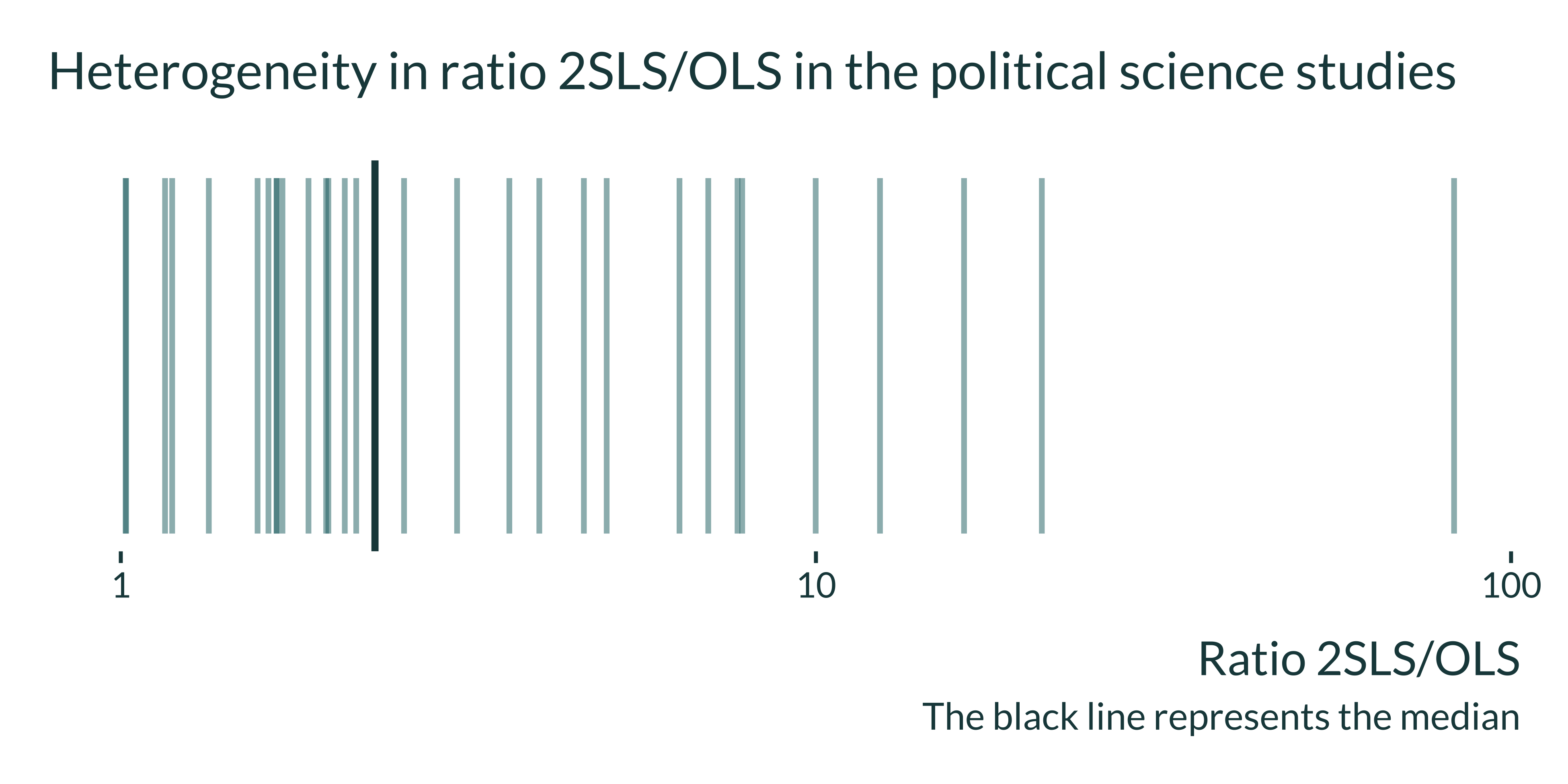
Power calculations
I then run similar power calculations as for Young (2022), computing what would be the statistical power and exaggeration if the true effect was equal to the OLS point estimate. Re
Show code
retro_lal_ols <- data_lal |>
  mutate(
    retro = map2(estimate_ols, se_iv, \(x, y) retro_design_closed_form(x, y))
    #retro_design returns a list with power, type_s, type_m
  ) |>
  unnest_wider(retro) |>
  mutate(power = power * 100)

summary_power(retro_lal_ols, lint_names = TRUE) |>
  mutate(results = "all", .before = 1) |>
  rename_with(\(x) str_to_title(str_replace_all(x, "_", " "))) |>
kable()| Results | Median Exagg | 3rd Quartile Exagg | Prop Exagg Larger Than 2 (%) | Median Power | 3rd Quartile Power |
|---|---|---|---|---|---|
| all | 2.1 | 5.1 | 61.3 | 23.3 | 31.4 |
Assuming that the true effects are half of the obtained estimates unsurprisingly yield similar results:
Show code
retro_lal_half <- data_lal |>
  mutate(
    retro = map2(estimate_iv/2, se_iv, \(x, y) retro_design_closed_form(x, y))
    #retro_design returns a list with power, type_s, type_m
  ) |>
  unnest_wider(retro) |>
  mutate(power = power * 100)

summary_power(retro_lal_half, lint_names = TRUE) |>
  mutate(results = "all", .before = 1) |>
  rename_with(\(x) str_to_title(str_replace_all(x, "_", " "))) |>
kable()| Results | Median Exagg | 3rd Quartile Exagg | Prop Exagg Larger Than 2 (%) | Median Power | 3rd Quartile Power |
|---|---|---|---|---|---|
| all | 1.9 | 2.3 | 41.9 | 27.1 | 40.2 |