Show the packages used in this document
library(tidyverse)
library(knitr)
library(mediocrethemes)
library(here)
library(retrodesign)
library(haven)
library(DT)
library(kableExtra)

set_mediocre_all(pal = "coty")
Approach and Data
Approach and Limitations
Brodeur, Cook, and Heyes (2020) assesses selection on significance in the universe hypothesis tests reported in articles published in 2015 and 2018 in the 25 top economics journals and using RCT, DID, RDD or IV. I leverage this data to investigate statistical power and exaggeration in this literature and then compare them across methods.
To do so, I first run a naive analysis: I explore whether the design of each study would enable to retrieve the true effect if it was twice smaller that the one found in the study.
There is no a priori reason to believe that the magnitude of the true effect of a specific study would be half of that of the estimate and not the estimate obtained. I am not claiming that these would be the true effect. Rather, I wonder what would be the power and exaggeration under this reasonable assumption, Ioannidis, Stanley, and Doucouliagos (2017) finding a typical exaggeration of two in the economics literature. This approach is also to some extent conservative: hypothesized effect sizes based on exaggerated estimates will be too large and will thus minimize exaggeration.
Note that Gelman and Carlin (2014), the seminal article on exaggeration, warns against using estimates from the study as true effects since they might be exaggerated. It instead recommends using estimate from other studies or meta analyses. Since meta-analyses estimates are not readily available for the studies in Brodeur, Cook, and Heyes (2020), I however run an analysis where hypothetical true effects are based on the published estimates. Even though the approach can be discussed, it allows a quick analysis of a very broad literature, in particular comparing the vulnerability of various studies.
In this document, I explore potential exaggeration of significant estimates. I exclude non-significant as they have not been selected on significance.1 This also allows abstracting from specifications for which significance was not even an objective (placebo tests or when trying to show an absence of effect).
Data
To run the analysis, I first retrieve the Brodeur, Cook, and Heyes (2020) data from OPENIPCSR and store it locally. I load it and wrangle it. The authors fixed some of their data after the publication of the article (changes explained in the Changelog.txt file). I keep the most recent data.
data_brodeur_raw <- read_dta(here("inputs", "brodeur_v2", "data", "MM Data.dta"))

data_brodeur <- data_brodeur_raw |>
  mutate(
    estimate = ifelse(!is.na(mu_new), mu_new, mu_orig),
    estimate = abs(estimate), #sign does not matter here
    se = ifelse(!is.na(sd_new), sd_new, sd_orig)
  ) |>
  group_by(title) |>
  mutate(article_id = cur_group_id()) |>
  ungroup() |>
  select(method, estimate, se, article_id) |>
  filter(se > 0) |>
  mutate(
    signif = (abs(estimate) > qnorm(0.975)*se)
  )
Brief exploratory data analysis
After some filtering, there are 20561 estimates with associated p-values from 646 articles. 10025 of these estimates are significant at the 5% confidence level. The distribution of the number of articles across journals is as follows:
Show the code used to generate the table
data_brodeur_raw |>
  select(journal, title) |>
  distinct() |>
  count(journal) |>
  arrange(desc(n)) |>
  kbl(col.names = c("Journal", "Number of articles")) |>
  kable_paper(c("hover"), html_font = "Lora") |>
scroll_box(width = "100%", height = "350px") | Journal | Number of articles |
|---|---|
| Journal of Public Economics | 74 |
| Journal of Development Economics | 64 |
| American Economic Review | 55 |
| Review of Economics and Statistics | 49 |
| AEJ: Applied Economics | 46 |
| AEJ: Economic Policy | 42 |
| Journal of Financial Economics | 40 |
| Review of Financial Studies | 39 |
| Economic Journal | 38 |
| Journal of Finance | 27 |
| Journal of Urban Economics | 26 |
| Quarterly Journal of Economics | 23 |
| Journal of Human Resources | 21 |
| Journal of Labor Economics | 20 |
| Journal of the European Economic Association | 20 |
| Journal of International Economics | 19 |
| Journal of Political Economy | 18 |
| Journal of Financial Intermediation | 16 |
| Econometrica | 10 |
| Journal of Economic Growth | 8 |
| Review of Economic Studies | 7 |
| Economic Policy | 6 |
| Experimental Economics | 6 |
| AEJ: Macroeconomics | 5 |
| Journal of Applied Econometrics | 5 |
The breakdown of the number of significant estimates by causal methods is:
Show the code used to generate the table
| Method | Number of estimates | Number of significant estimates |
|---|---|---|
| DID | 5464 | 3117 |
| IV | 4822 | 2800 |
| RCT | 7186 | 2720 |
| RDD | 3089 | 1388 |
| Total | 20561 | 10025 |
Overall power assessment
I then explore the power of the literature to retrieve effects whose magnitude would be equal to half the published estimate, using the retrodesign package. The preferred results are the ones restricted to the 10025 statistically significant estimates.
retro_brodeur <- data_brodeur |>
  mutate(
    retro = map2(estimate/2, se, \(x, y) retro_design_closed_form(x, y))
    #retro_design returns a list with power, type_s, type_m
  ) |>
  unnest_wider(retro) |>
  mutate(power = power * 100, type_s = type_s * 100)

retro_brodeur_signif <- retro_brodeur |>
  filter(signif)
For this hypothetical effect size, we have:
Show code
| Results | Median Exagg | 3rd Quartile Exagg | Prop Exagg Larger Than 2 (%) | Median Power | 3rd Quartile Power |
|---|---|---|---|---|---|
| All | 2.6 | 5.5 | 65.3 | 15.8 | 36.6 |
| Significant | 1.6 | 2.1 | 28.8 | 37.7 | 72.8 |
The overall distribution of power for significant estimates is:
Show code
retro_brodeur_signif |>
  ggplot(aes(x = power)) +
  # geom_density() +
  geom_histogram(bins = 100) +
  labs(
    title = "Distribution of power in the causal inference literature",
    subtitle = "Assuming a true effect size equal to half of the obtained estimate",
    x = "Power",
    y = "Count",
    caption = "There are no design with very low power because insignificant results were filtered out"
  ) +
xlim(c(0, NA)) 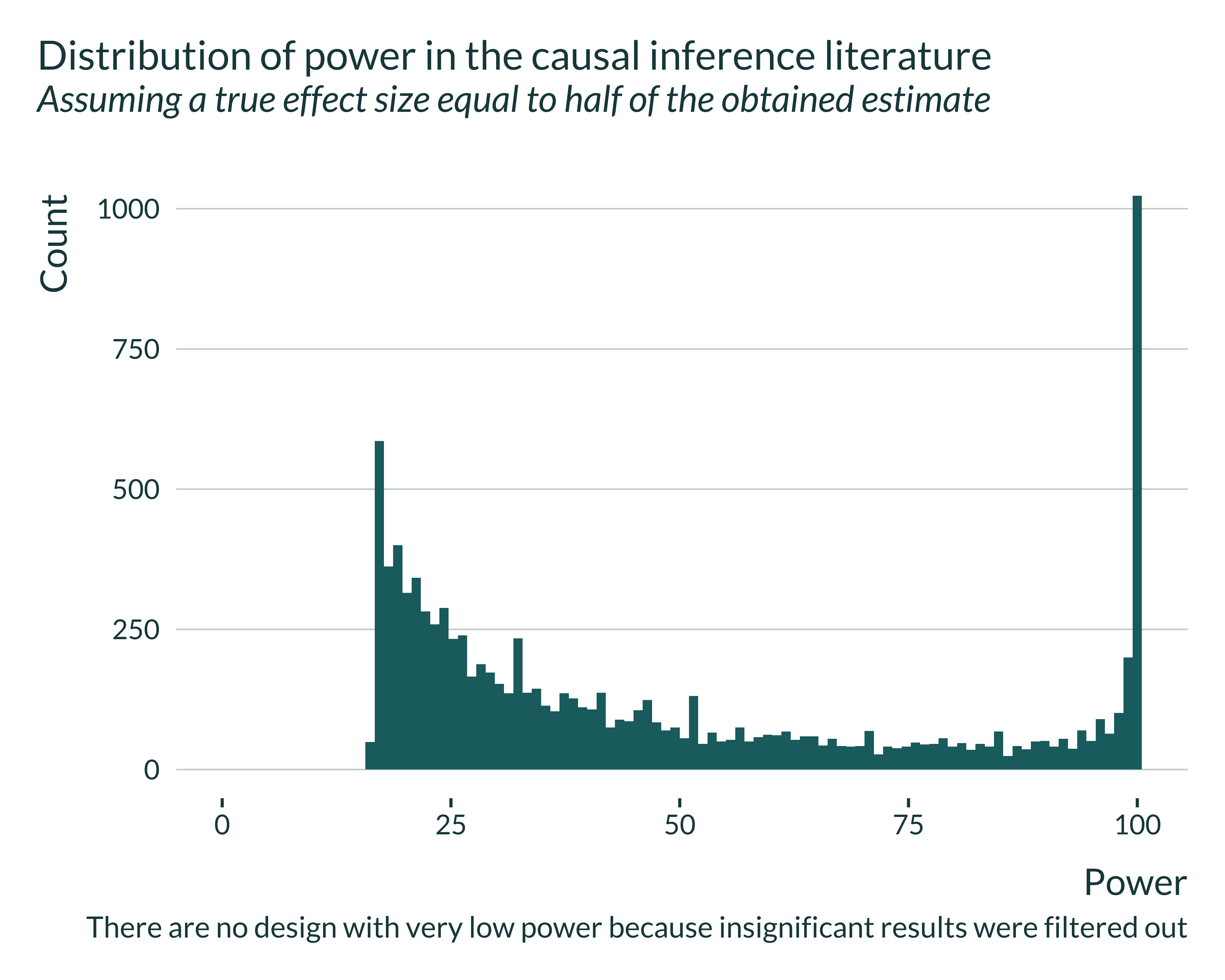
This figure underlines clear heterogeneity across designs. A substantial share of these designs have more than 99% power to detect such effect (11% of designs). Yet, only 22% of these designs would have a power greater than the conventional 80% threshold. For one quarter of the studies, exaggeration would be greater than 2.1.
Interestingly, restricting the sample to significant results, while the median power of to detect the estimate obtained itself would be 91%, only 63% of estimates would have a power greater to detect the estimate found in the analysis.
Power issues do not therefore concern all designs but can be substantial for some of them.
Importantly, type-S does not seem to be a important concern here:
Show code
retro_brodeur_signif |>
  ggplot(aes(x = type_s)) +
  # geom_density() +
  geom_histogram(bins = 50) +
  labs(
    title = "Distribution of type-S in the causal inference literature",
    subtitle = "Assuming a true effect size equal to half of the obtained estimate",
    x = "Type S (%)",
    y = "Count"
  ) +
  xlim(c(-0.3, 10))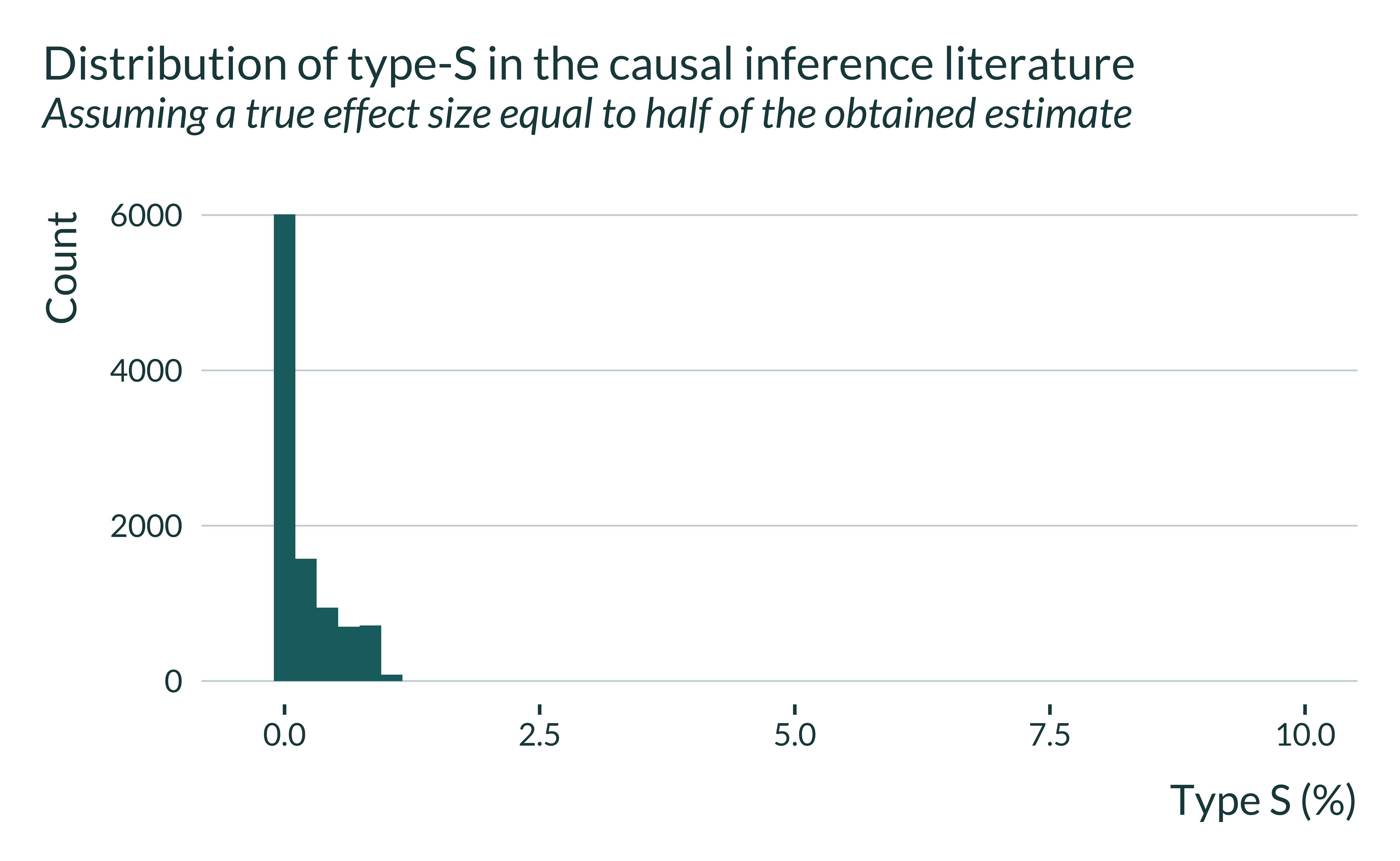
Comparison across methods
I then explore differences in exaggeration across methods. There are two ingredients in the recipe for exaggeration:
- Selection on significance
- Low statistical power
In order to explore whether some causal identification methods are more prone to exaggeration than others, we can thus explore which ones are more subject to each of these ingredients.
Differences of publication bias across methods
Studying differences across methods in terms of selection on significance is the main goal of Brodeur, Cook, and Heyes (2020). The paper shows that IV and to a lesser extent DiD are particularly problematic in this regard. RDD and RCT seem to be less prone to this issue.
Differences of statistical power and exaggeration across methods
I decompose the analysis carried above by identification strategy. For each identification strategy, the median power and exaggeration is:
Show the code used to generate the table
retro_brodeur_signif |>
  group_by(method) |>
  summarise(
    median_exagg = median(type_m),
    median_power = median(power),
    sd_of_power = sd(power),
    percent_adequate_power = mean(power > 80)*100
  ) |>
  rename_with(\(x) str_to_title(str_replace_all(x, "_", " "))) |>
kable()| Method | Median Exagg | Median Power | Sd Of Power | Percent Adequate Power |
|---|---|---|---|---|
| DID | 1.547748 | 40.98285 | 29.32969 | 23.54828 |
| IV | 1.637126 | 36.53802 | 28.67865 | 20.14286 |
| RCT | 1.677622 | 34.78188 | 29.14046 | 20.99265 |
| RDD | 1.601895 | 38.19035 | 29.72434 | 22.33429 |
There does not seem to be substantial differences in medians. If anything, RCT seem to perform slightly less well than the others and DID slightly better.
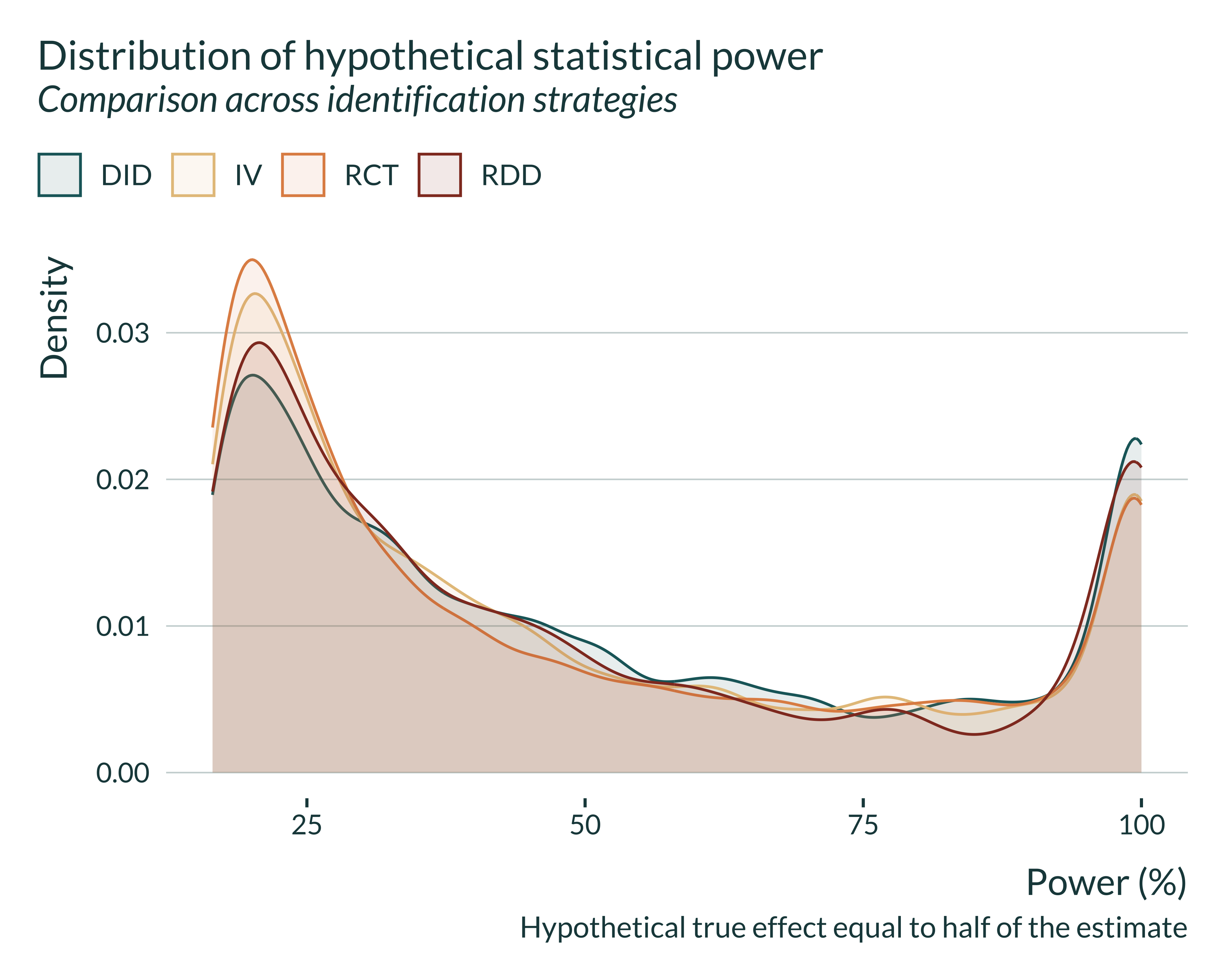
The distributions of power and exaggeration, by methods, are:
Show the code used to generate the graph
retro_brodeur_signif |>
  ggplot(aes(x = power, fill = method, color = method)) +
  geom_density(alpha = 0.1, adjust = 0.5) +
  # facet_wrap(~method, scales = "free_y") +
  labs(
    title = "Distribution of hypothetical statistical power",
    subtitle = "Comparison across identification strategies",
    x = "Power (%)",
    y = "Density",
    caption = "Hypothetical true effect equal to half of the estimate",
    fill = NULL,
    color = NULL
  )
Show the code used to generate the graph
retro_brodeur_signif |>
  # filter(exagg < 3) |>
  ggplot(aes(x = type_m, fill = method, color = method)) +
  geom_density(alpha = 0.1) +
  # facet_wrap(~method) +
  labs(
    title = "Distribution of hypothetical exaggeration",
    subtitle = "Comparison across identification strategies",
    x = "Exaggeration ratio",
    y = "Density",
    caption = "Hypothetical true effect equals to half of the estimate",
    fill = NULL,
    color = NULL
  )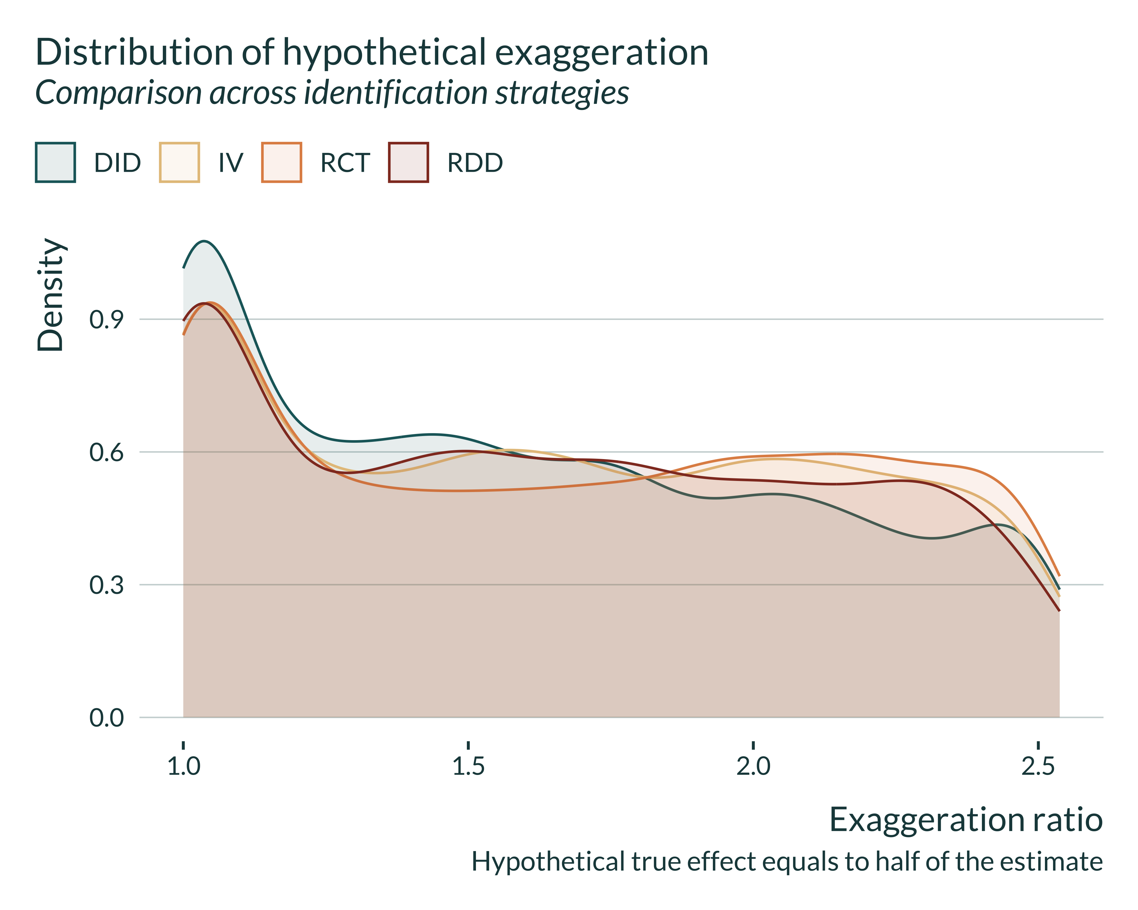
The results are rather similar across strategies. If anything, we notice that DID performs slightly better. However, if there is initially more exaggeration for one of the methods, considering hypothetical true effect sizes equal to half of the observed estimates would attenuate this difference.
Note that this exclusion is conservative.↩︎