Show code to load packages

library(rmarkdown) 
library(knitr) 
library(here) 
library(tidyverse)
library(missRanger) 
library(mediocrethemes) #own ggplot theme

set_mediocre_all(pal = "leo")

Selecting Cities with the Least Proportion of Missing Observations

First, we load the data. We then notice in the exploratory data analysis that average temperature readings were missing for all cities after 1998. We therefore select observations from 1987 to 1997:

nmmaps_to_clean <- readRDS(here::here("data", "clean_data", "nmmaps_data.rds"))

nmmaps_filtered <- nmmaps_to_clean %>%
  filter(date <= "1997-12-31")

We select cities with less than 5% of missing temperature readings:

cities_to_keep <- nmmaps_filtered %>%
  group_by(city) %>%
  summarise(proportion_missing = sum(is.na(temperature))/n()*100) %>%
  filter(proportion_missing<=5) %>%
  pull(city)

nmmaps_filtered <- nmmaps_filtered %>%
  filter(city %in% cities_to_keep)

We will only use the carbon monoxide in our power simulations as it is the pollutant with the smallest proportion of missing readings. We keep cities with less than 5% of missing CO readings:

cities_to_keep <- nmmaps_to_clean %>%
  group_by(city) %>%
  summarise(proportion_missing = sum(is.na(co))/n()*100) %>%
  filter(proportion_missing<=5) %>%
  pull(city)

nmmaps_to_clean <- nmmaps_to_clean %>%
  filter(city %in% cities_to_keep)

We have 66 cities remaining. We plot the proportion of missing values for CO by city:

Show code

nmmaps_to_clean %>%
  group_by(city) %>%
  summarise(proportion_missing = sum(is.na(co))/n()*100) %>%
  arrange(proportion_missing) %>%
  mutate(city = factor(city, levels = city)) %>%
  ggplot(., aes(x = proportion_missing, y = city)) +
  geom_vline(xintercept = sum(is.na(nmmaps_to_clean$co))/nrow(nmmaps_to_clean)*100) +
  geom_point(size = 3) +
  xlab("Proportion of Missing Values (%)") + 
  ylab(NULL)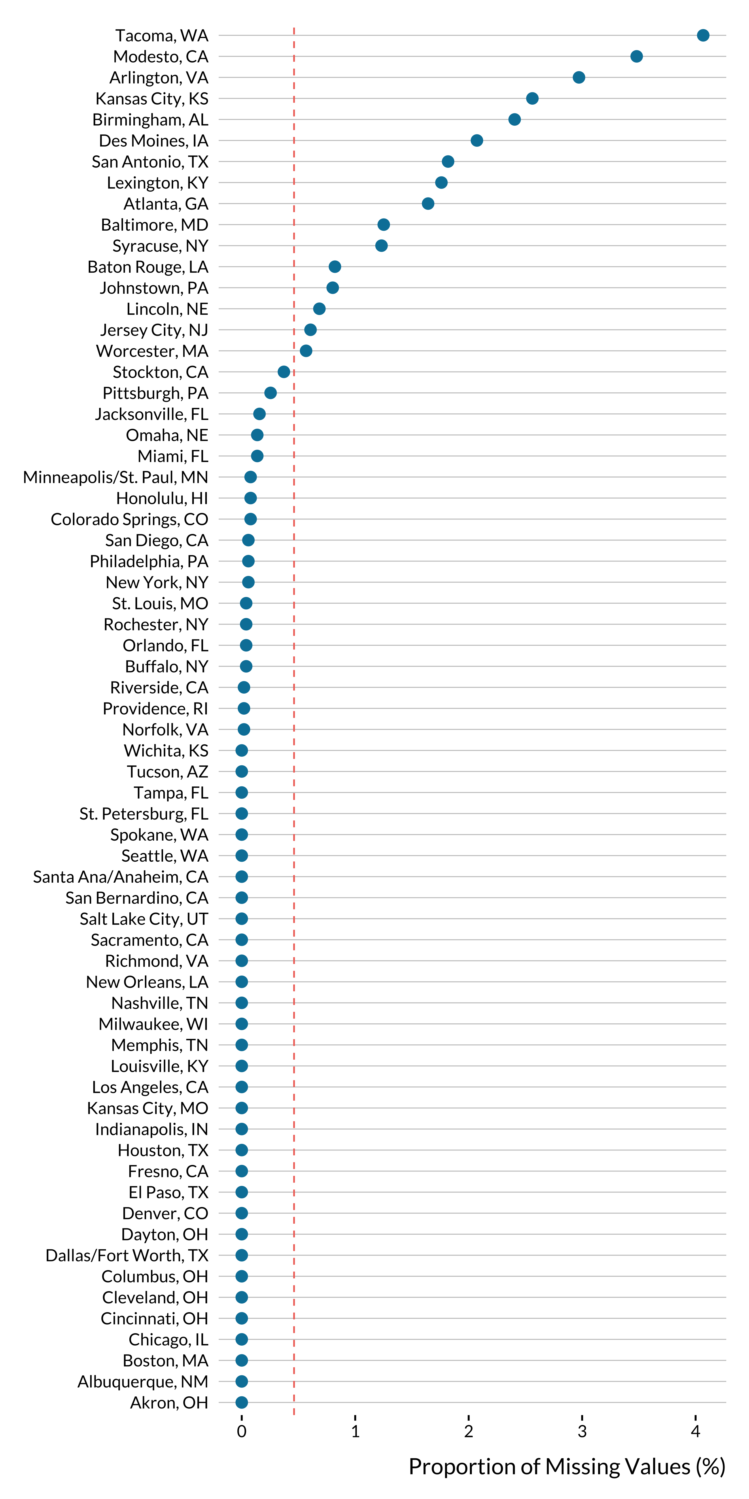

We also plot the time series of missing values for CO by city:

Show code

nmmaps_to_clean %>%
  mutate(missing_co = ifelse(is.na(co), "Missing", "Not Missing")) %>%
  ggplot(., aes(x = date, y = city, fill = fct_rev(missing_co))) +
  geom_tile() +
  scale_x_date(breaks = scales::pretty_breaks(n = 6)) +
  labs(
    x = "Date",
    y = NULL,
    fill = NULL
  ) + 
  theme(panel.grid.major.y = element_blank(),
        legend.justification = "left",
        axis.text.y = element_text(margin = margin(r = -0.5, unit = "cm")))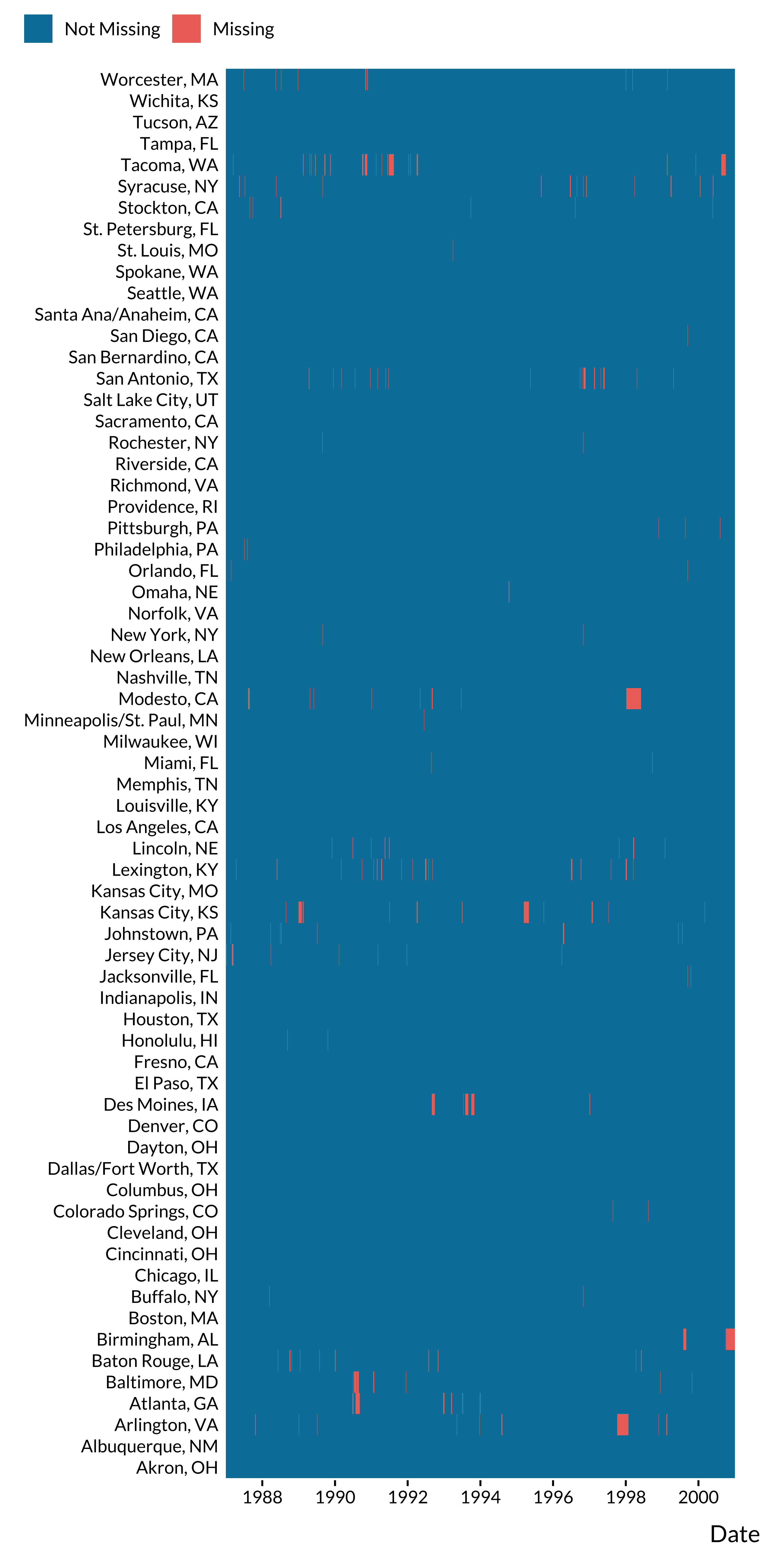

The overall distribution of CO in \(\mu g/m^{3}\) is as follows:

Show code

nmmaps_to_clean %>%
  summarise(Mean = mean(co, na.rm = TRUE),
            "Standard Deviation" = sd(co, na.rm = TRUE),
            Minimum = min(co, na.rm = TRUE),
            Maximum = max(co, na.rm = TRUE)) %>%
  kable(.)

Mean	Standard Deviation	Minimum	Maximum
369.2361	398.3864	1.03e-05	8335.371

We impute missing observations for CO concentrations and the average temperature using the missRanger package:

We scale (“standardize”) the CO concentrations:

nmmaps_data_simulations <- nmmaps_imputed %>%
  mutate(co = scale(co) %>% as.vector)

We finally keep relevant variables and save the data:

nmmaps_data_simulations %>%
  select(city:temperature, co:resp_total) %>%
  mutate_at(vars(city, state, year), ~ as.factor(.)) %>%
  saveRDS(., here::here("data", "clean_data", "nmmaps_data_simulations.rds"))

We have 273224 observations, with 4018 daily observations by city.

Data Cleaning for Power Simulations

Selecting Cities with the Least Proportion of Missing Observations