In this document, we explore the relationship between the reported estimated effect sizes of air pollutants on health outcomes and the precision of these estimates in the epidemiology literature. Since our automated search of the literature does not allow us to easily standardize estimates, we rely on two recently published meta-analysis by Orellano et al. (2020) and Shah et al. (2015) whose data are openly available:
- Orellano et al. (2020) selected 196 studies on the short-term associations between air pollutants and mortality for all causes but also for specific causes. Their data are available in the Supplementary Files they provided.
- Shah et al. (2015) gathered 94 studies on the short-term associations between air pollutants and admission to hospital or mortality due to stroke. Their data are available in the “Appendix six - Individual forest plots for each pollutant” of the Data Supplement.
Compared to the causal inference literature on this topic, the “standard” epidemiology literature is much more homogeneous since it has produced many studies with very similar designs (i.e., same statistical model, same specification, same health outcome, etc.).
For each study of these two datasets, we also compute their statistical power, type M and S errors using the results of the meta-analysis as guesses for the true effect sizes of an air pollutant on an health outcome.
Loading Packages and Data
Show the packages used
library("groundhog")
packages <- c(
  "here",
  "tidyverse",
  "knitr",
  "retrodesign",
  "janitor",
  "mediocrethemes"
  # "vincentbagilet/mediocrethemes"
)

# groundhog.library(packages, "2022-11-28")
lapply(packages, library, character.only = TRUE)

set_mediocre_all(pal = "leo")
We open the two meta-analysis datasets and clean them.
Show code
data_orellano_2020 <-
  read_csv(here::here(
    "data",
    "meta_analyses_epi",
    "meta_analysis_orellano_2020.csv"
  )) |>
  janitor::clean_names() |>
  # remove studies using the one hour maximum concentration of no2
  mutate(time_period = ifelse(is.na(time_period), "unknown", time_period)) |>
  filter(time_period != "1 hr") |>
  select(
    article,
    continent,
    age_group,
    sex,
    pollutant,
    unit_measurement = unit_of_measurement,
    time_period,
    cause_death = cause_of_death,
    point_estimate = "single_pollutant_effect_estimate",
    lower_bound_ci = "single_pollutant_lower_interval_limit_95_percent_ci",
    upper_bound_ci = "single_pollutant_higher_interval_limit_95_percent_ci"
  ) |>
  mutate(year = str_extract(article, "[[:digit:]]+") %>% as.numeric(.))

data_shah_2015 <-
  readxl::read_excel(here::here("data", "meta_analyses_epi", "meta_analysis_shah_2015.xlsx")) %>%
  mutate(air_pollutant = str_to_upper(air_pollutant))
Orellano et al. (2020) Meta-Analysis
We start by exploring the studies gathered by Orellano et al. (2020) on the short-term associations between air pollutants and mortality for all causes and specific causes. We first select studies focusing mortality for all ages and sexes. We then compute our metric for precision, which the inverse of the standard error, and also calculate the width of the 95% confidence intervals:
Relative Risks versus Precision
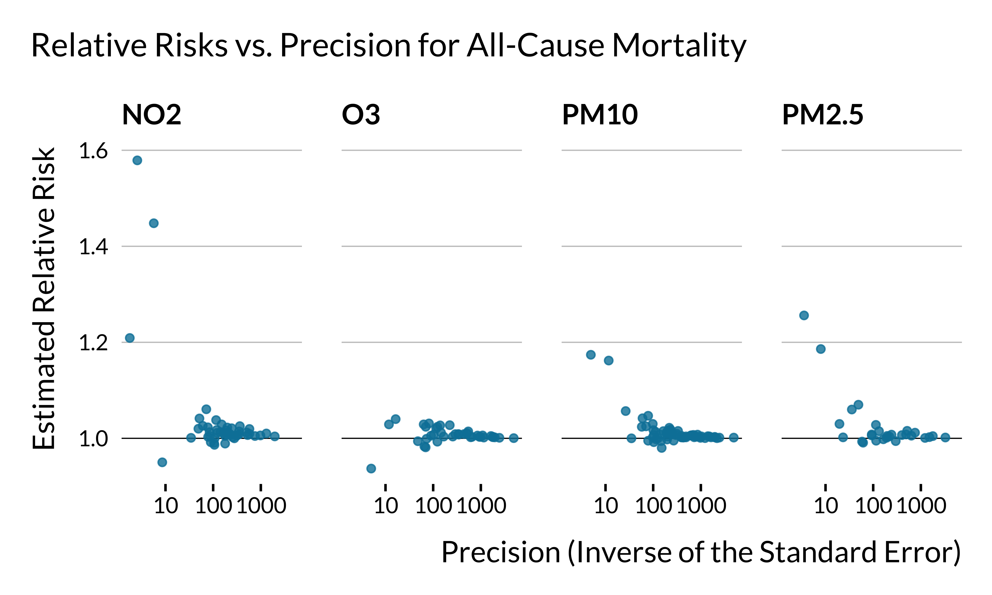
We plot below the relationship between estimated relative risks for all-cause mortality and precision for each air pollutant (N=176 estimates):
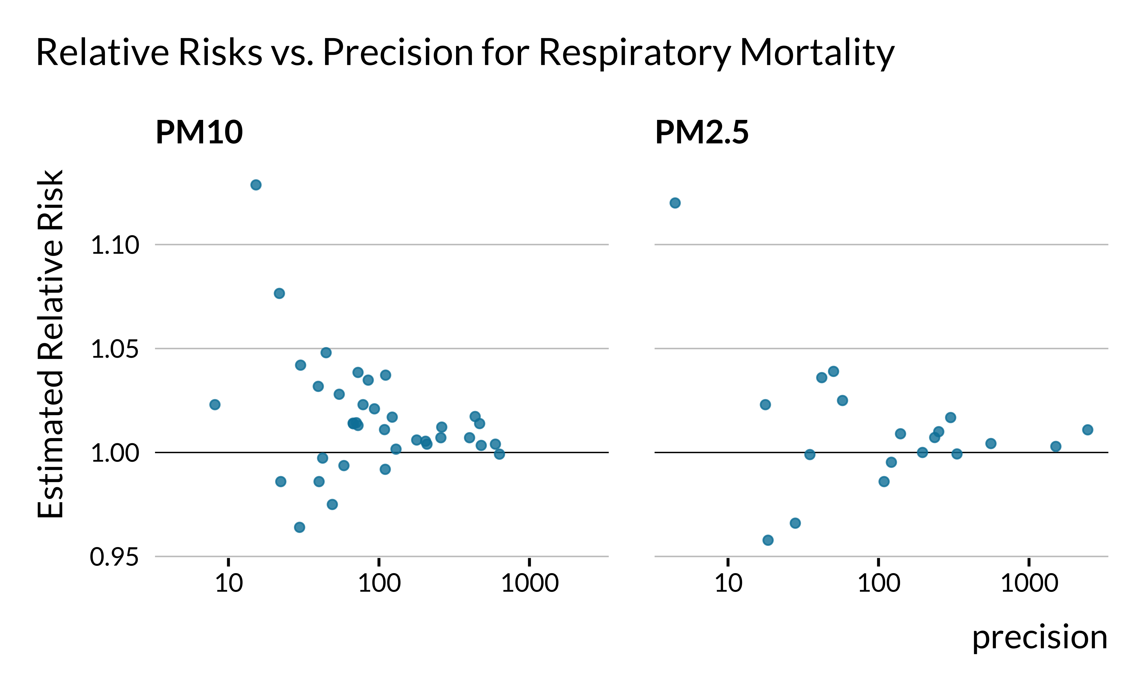
We draw the same initial graph but for respiratory mortality (N=56 estimates):
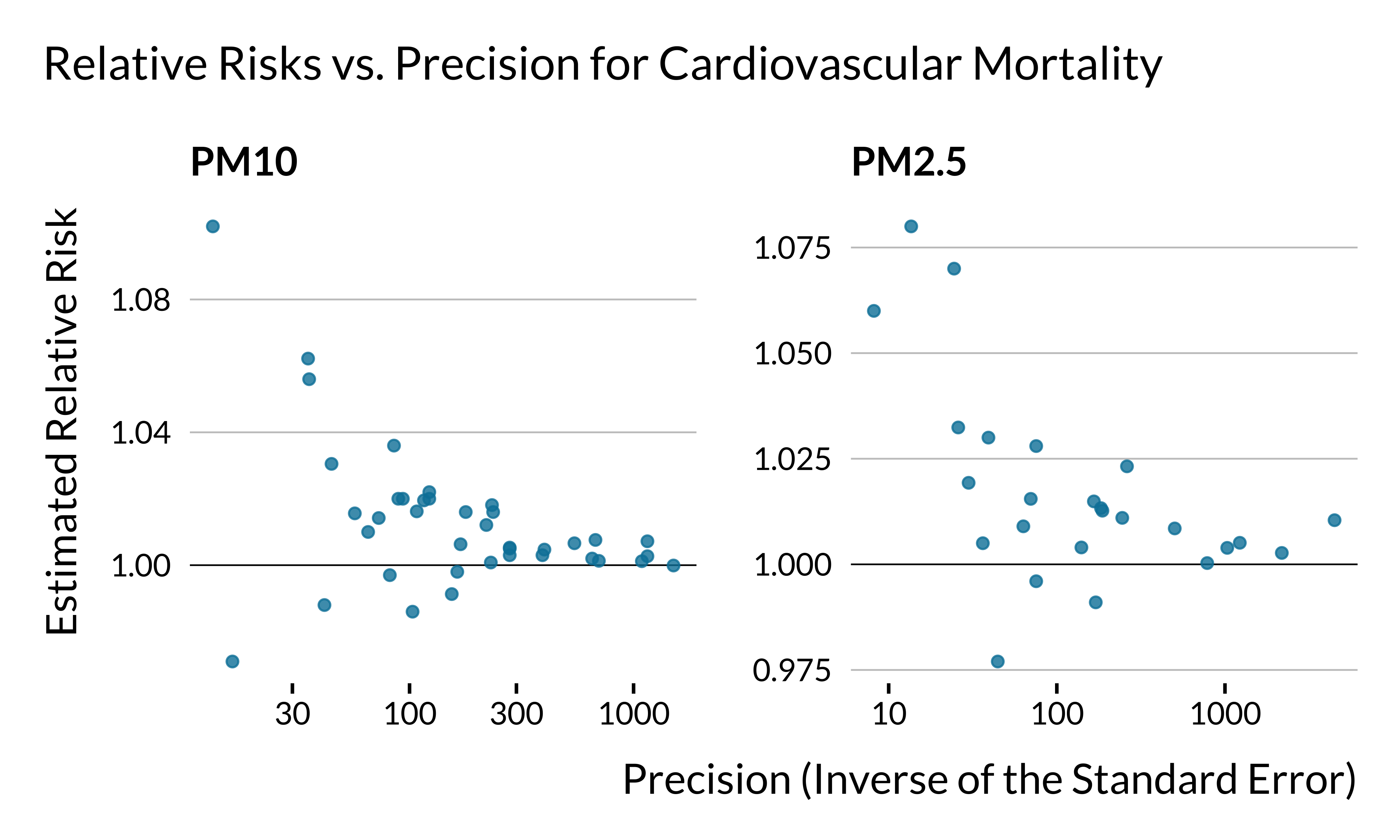
We draw the same previous graph but now for cardiovascular mortality (N=64 estimates):
Evolution of Precision over Time
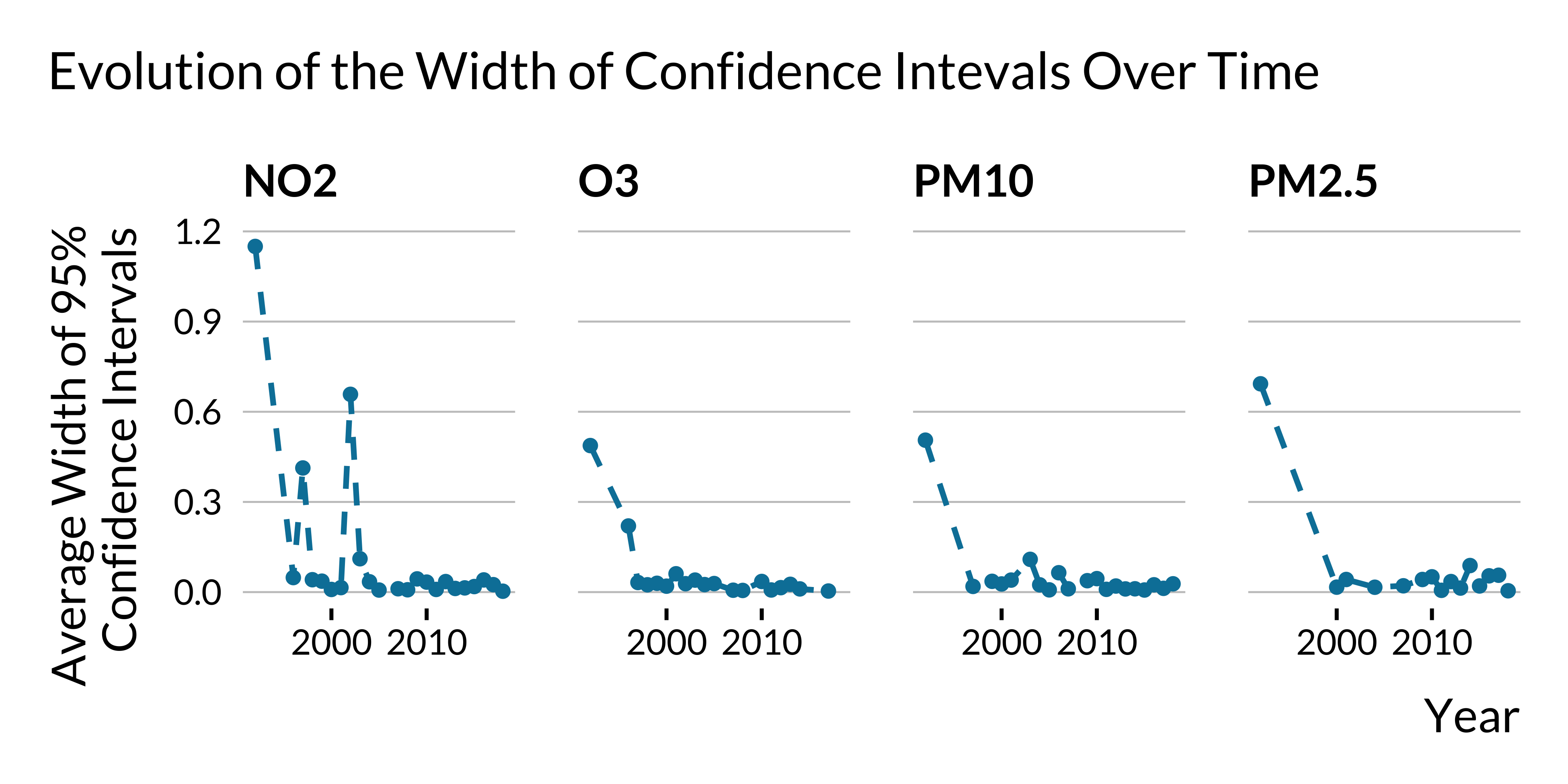
We plot below the mean width of 95% confidence intervals over time for estimated relative risks of all-cause mortality:
95% CI Width as a Percentage of Estimated Relative Risk
We finally display the distribution of the 95% CI width expressed as percentage of the estimated relative risk.
| Pollutant | Mean | Standard Deviation | Minum | Maximum |
|---|---|---|---|---|
| NO2 | 9 % | 23.9 % | 0.3 % | 138.6 % |
| O3 | 5 % | 12.1 % | 0.1 % | 71.2 % |
| PM10 | 3.5 % | 8.3 % | 0.1 % | 59.3 % |
| PM2.5 | 7.5 % | 15.3 % | 0.1 % | 74.6 % |
Results on PM\(_{10}\) are the more precise.
Computing Statistical Power, Type M and S errors
We compute in this section the statistical power, the probability to make a Type S error and the exaggeration factor (the average Type M error) for studies included in the meta-analysis. As a guess for the true effect size of each study, we extract the meta-analysis estimates displayed in the Table 1 of the article. We then rely on the https://github.com/andytimm/retrodesign package to compute the statistical power, type M and S error.
Two important remarks:
* We had to convert the estimates as percentage increases because the retrodesign() function does not work with relative risks (assuming a linear relationship, Orellano et al. (2020) use the following formula: Percentage Increase = (RR-1)$$100).
* We only consider studies that were initially deemed statistically significant at the 5% level.
We display below the median of the three metrics by air pollutant:
| Air Pollutant | Cause of Death | Number of Studies | Statistical Power (%) | Type M Error | Type S Error (%) |
|---|---|---|---|---|---|
| PM10 | Cerebrovascular | 8 | 20 | 3 | 2 |
| PM10 | Respiratory | 9 | 20 | 2 | 1 |
| PM10 | Cardiovascular | 14 | 22 | 2 | 0 |
| PM10 | All-cause | 31 | 36 | 2 | 0 |
| NO2 | All-cause | 25 | 46 | 1 | 0 |
| O3 | All-cause | 22 | 63 | 1 | 0 |
| PM2.5 | Cardiovascular | 11 | 67 | 1 | 0 |
| PM2.5 | Cerebrovascular | 2 | 69 | 1 | 0 |
| PM2.5 | Respiratory | 6 | 90 | 1 | 0 |
| PM2.5 | All-cause | 11 | 92 | 1 | 0 |
Shah et al. (2015) Meta-Analysis
In this section, we analyse the studies gathered by Shah et al. (2015) on the link between short-term exposure to air pollution and stroke hospital admission or mortality. As for the previous dataset, we compute our measure of precision and the width of 95% confidence intervals:
Relative Risks versus Precision
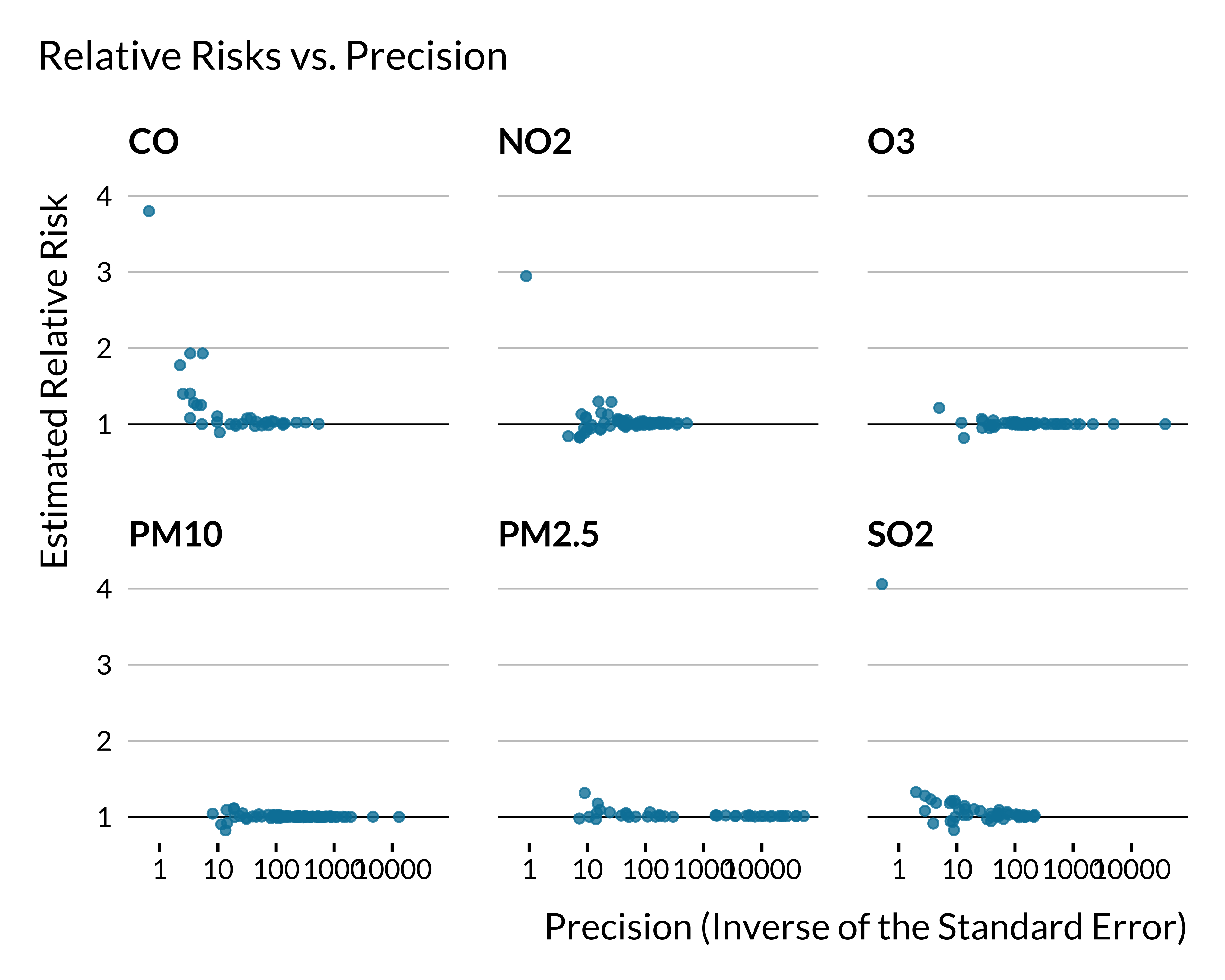
We plot below the relationship between estimated relative risks and precision for each air pollutant:
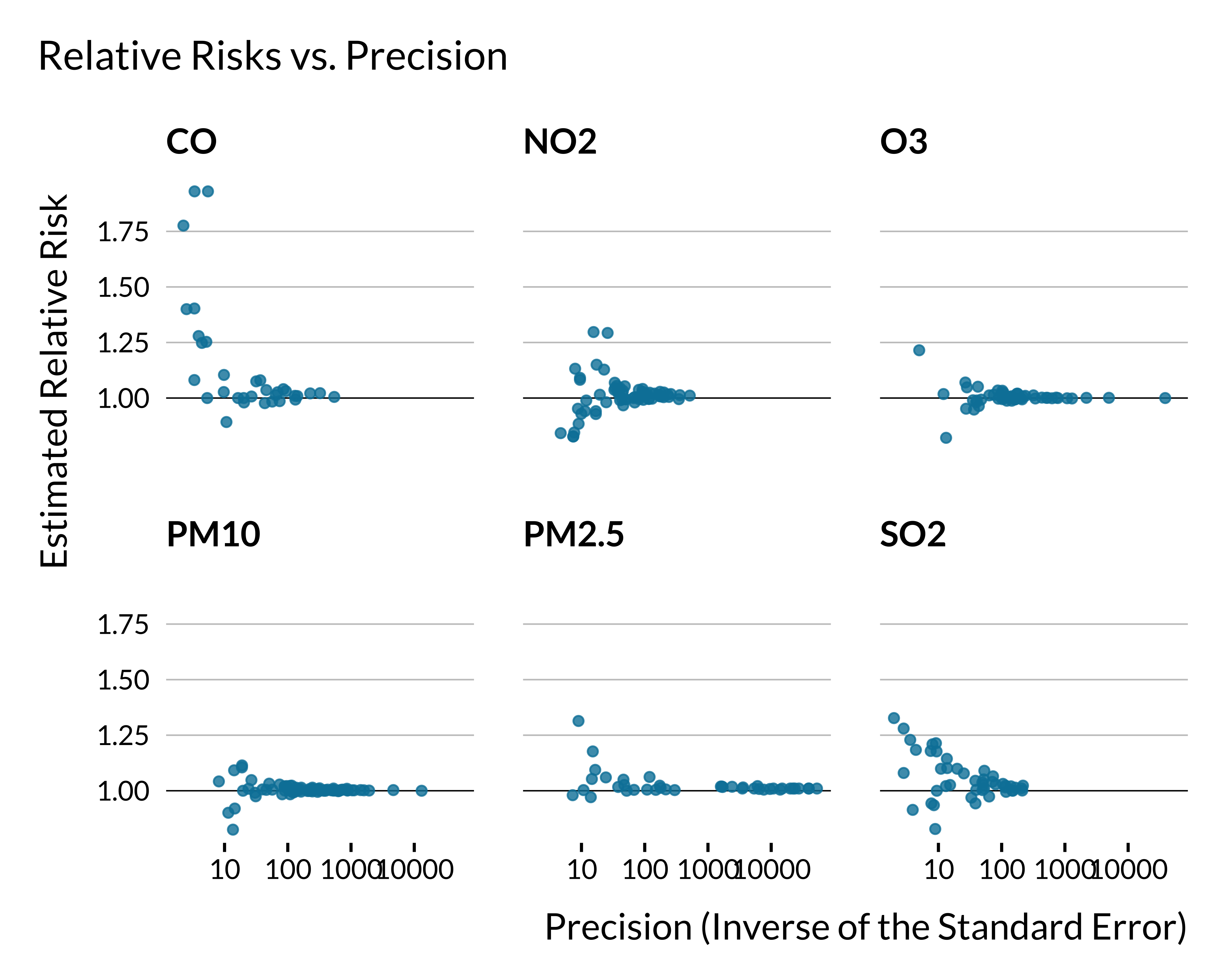
We plot the same figure but for estimated relative risks below 2:
Evolution of Precision over Time
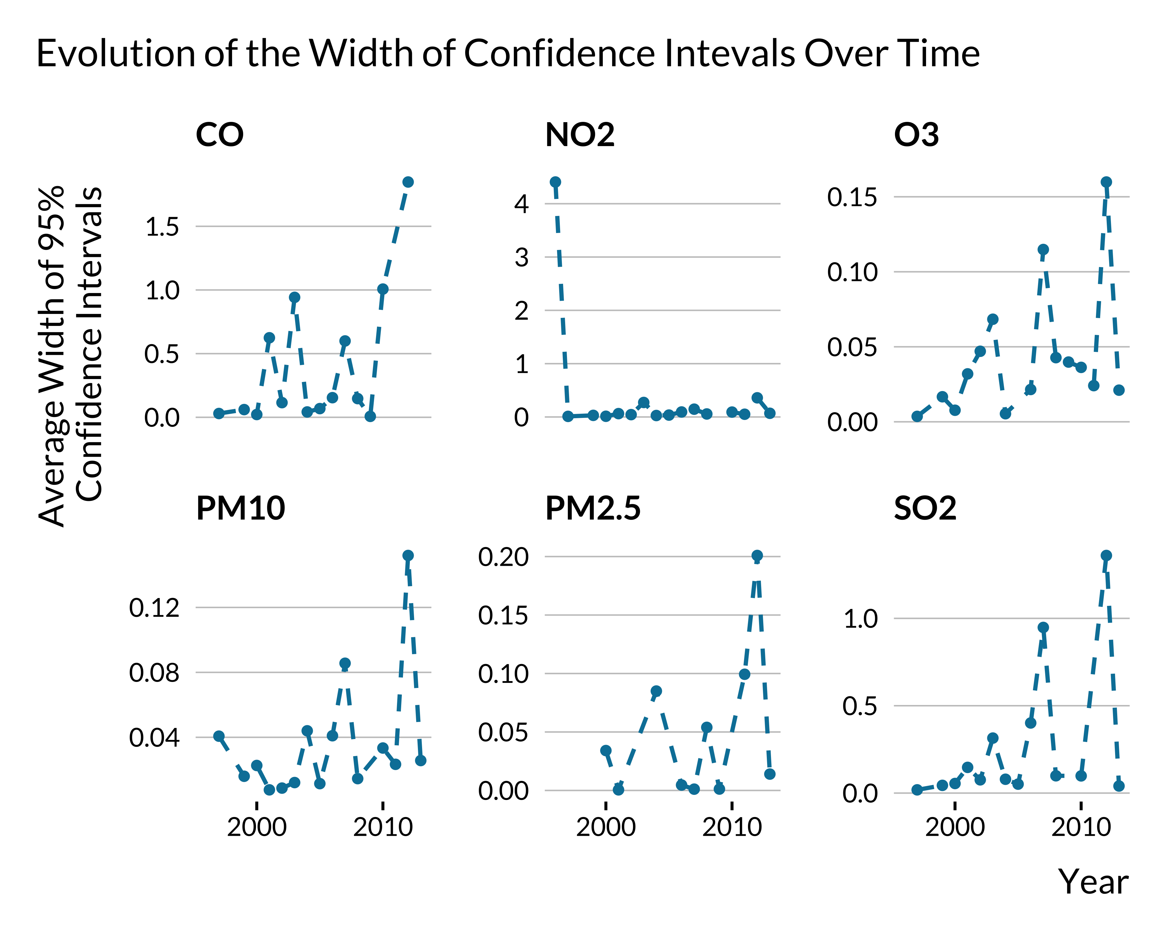
We plot below the mean width of 95% confidence intervals over time for estimated relative risks:
95% CI Width as a Percentage of Estimated Relative Risk
We finally display the distribution of the 95% CI width expressed as percentage of the estimated relative risk.
| Pollutant | Mean | Standard Deviation | Minum | Maximum |
|---|---|---|---|---|
| CO | 35.9 % | 40.6 % | 0.7 % | 158.2 % |
| NO2 | 17.2 % | 25.2 % | 0.8 % | 149.6 % |
| O3 | 6.3 % | 10.7 % | 0 % | 64.9 % |
| PM10 | 5.5 % | 9.1 % | 0 % | 46.3 % |
| PM2.5 | 7.2 % | 12.6 % | 0 % | 55.1 % |
| SO2 | 32.1 % | 42.8 % | 1.8 % | 187.6 % |
Computing Statistical Power, Type M and S errors
As a guess for the true effect size of each study, we extract the meta-analysis estimates displayed in the Figure 1 of the article. We then rely on the https://github.com/andytimm/retrodesign package to compute the statistical power, type M and S error.
We display below the median of the three metrics by air pollutant:
| Air Pollutant | Statistical Power (%) | Type M Error | Type S Error (%) |
|---|---|---|---|
| CO | 41 | 10 | 11 |
| NO2 | 42 | 3 | 5 |
| O3 | 18 | 17 | 28 |
| PM10 | 39 | 7 | 9 |
| PM2.5 | 83 | 3 | 3 |
| SO2 | 50 | 2 | 1 |
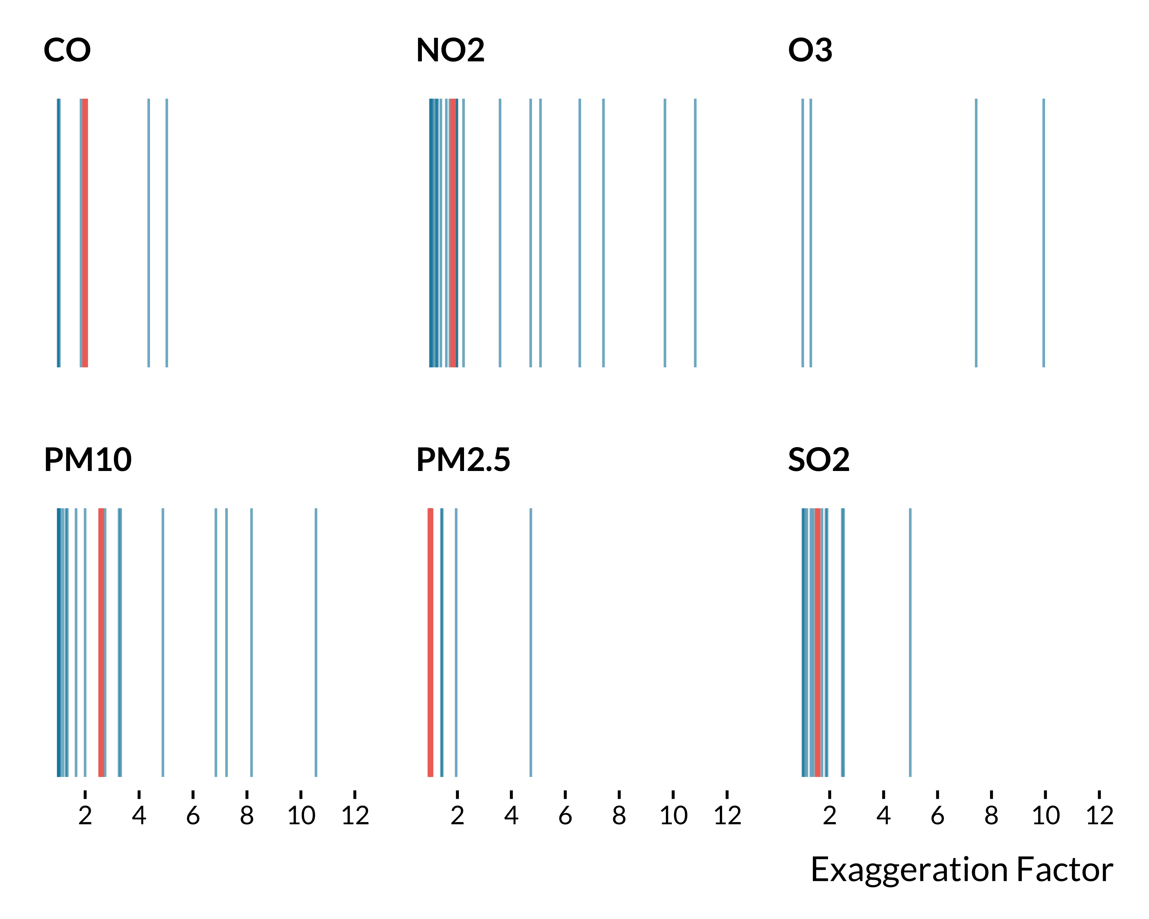
We display below the distribution of the exaggeration ratio by air pollutant: