This document focuses on actually running the simulations. The overall approach to the simulations is described here and the results are analyzed and discussed here.
Show the packages used
library("groundhog")
packages <- c(
  "here",
  "tidyverse",
  "knitr",
  "broom",
  "lubridate",
  "tictoc",
  "rlang",
  "readr",
  "fixest",
  "Formula",
  "furrr",
  "progress",
  "progressr",
  "mediocrethemes"
  # "vincentbagilet/mediocrethemes"
)

# groundhog.library(packages, "2022-11-28")
lapply(packages, library, character.only = TRUE)

set_mediocre_all(pal = "leo")

# Settings for progress bar
handlers(list(
  handler_progress(
    format   = ":spin :current/:total (:message) [:bar] :percent in :elapsed ETA: :eta"
  )
))

nmmaps_data <- readRDS(
    here::here("data", "simulations", "nmmaps_data_simulations.rds")
  ) %>%
  mutate(temperature_squared = temperature^2)
Function definitions
Selecting the study period
First, we create a function to randomly select a study period of a given length. This function also randomly selects a given number of cities to consider. For simplicity, we choose to have the same temporal study period for each city. This also seems realistic; a study focusing on several cities would probably consider a unique study period.
This function randomly selects a starting date for the study, early enough so that the study can actually last the number of days chosen. It then randomly draws a given number of cities and filters out observations outside of the study period. It returns a data set with only the desired number of cities and days.
select_study_period <- function(data, n_days = 3000, n_cities = 68) {
  dates <- data[["date"]]
  err_proof_n_days <- min(n_days, length(unique(dates)))
  cities <- data[["city"]]
  err_proof_n_cities <- min(n_cities, length(unique(cities)))

  begin_study <- sample(
    seq.Date(
      min(dates),
      max(dates) - err_proof_n_days,
      "day"
    ), 1)

  dates_kept <- dplyr::between(
    dates,
    begin_study,
    begin_study + err_proof_n_days
  )

  cities_kept <- cities %in% sample(levels(cities), size = err_proof_n_cities)

  data_study <- data[(dates_kept & cities_kept),]
  return(data_study)
}
Defining the treatment
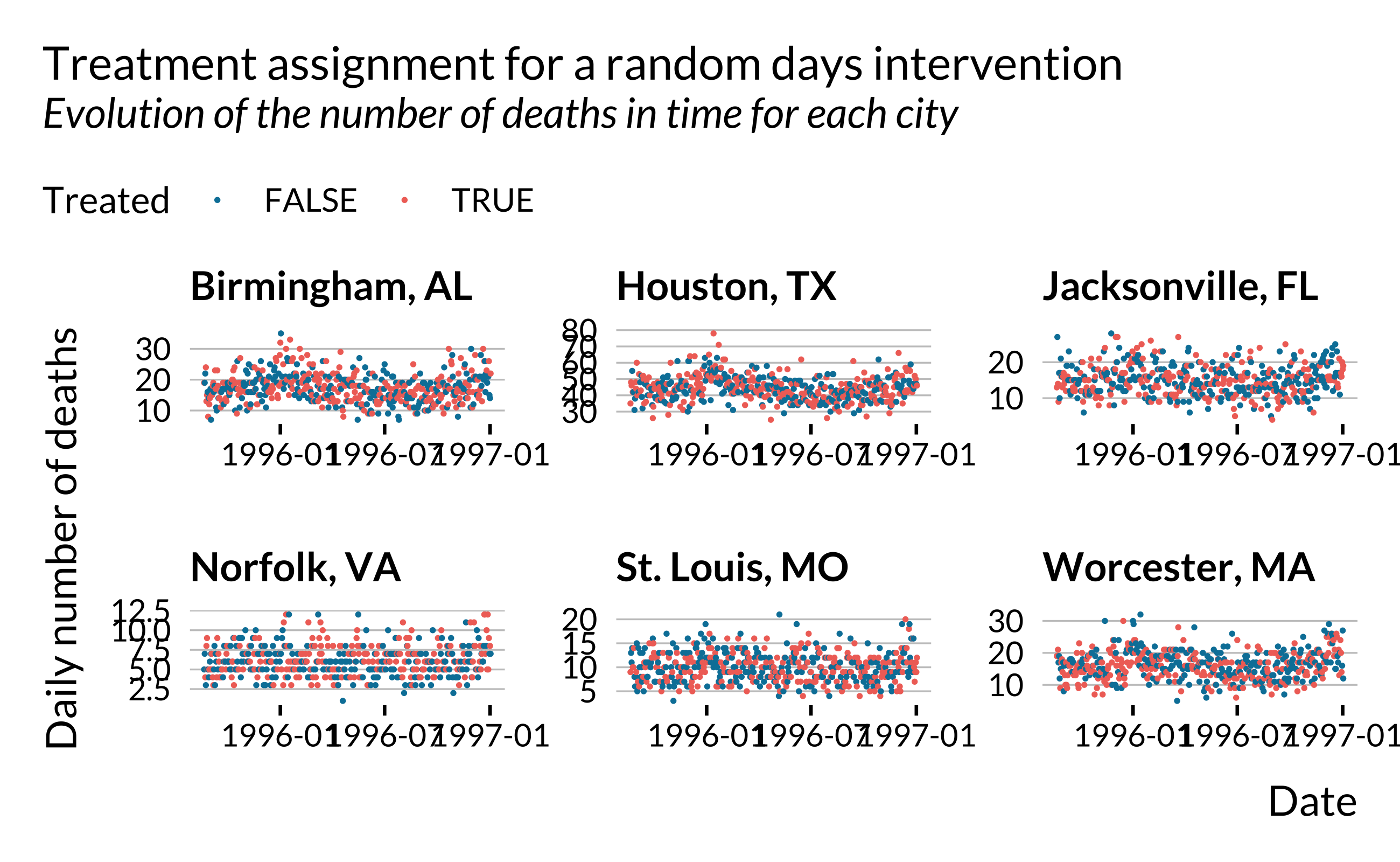
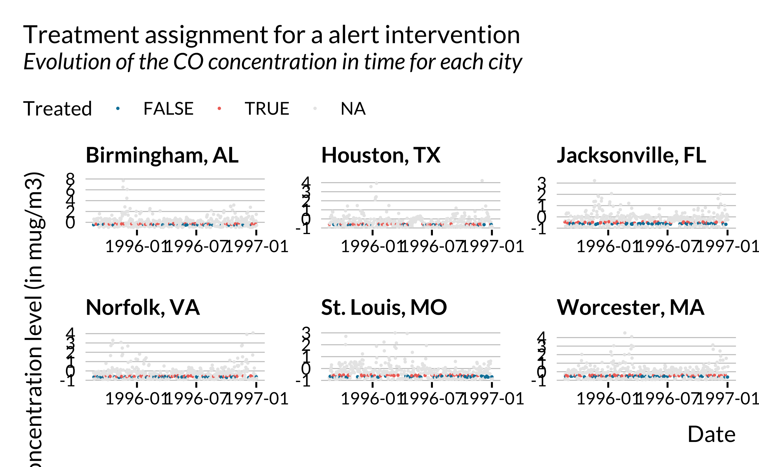
Then, we create a function to draw the treatment. This function adds a boolean vector to our data, stating whether each observation is in the treatment group or not. The drawing procedure depends on the quasi experiment considered (quasi_exp) and the proportion of treated observations (p_obs_treat). We consider three quasi-experiments:
- Random days, corresponding to a random allocation of the treatment (
random_days) - Air pollution alerts (
alert_...with … being the pollutant name ) - No quasi-experiment (
none)
Note that for the alert, we will use RDD to estimate the effect of the treatment. We therefore restrict our sample to observations in a given bandwidth. We draw a threshold position from a uniform distribution from 0.2 to 0.4 in order to have enough observations in our data set. If we pick the threshold position too high up in the distribution of CO concentration, we may end up with observations very far away from the samples. For each city, we find the corresponding threshold and define a bandwidth such that p_obs_treat observations of the total sample are treated. Observations outside the bandwidth get a NA for treated. Thus, after calling this function, we need to filter out observations with a NA for treated.
draw_treated <- function(data, p_obs_treat = 0.5, quasi_exp = "random_days") {

  if (quasi_exp == "random_days") {
    data[["treated"]] <- rbernoulli(length(data[["date"]]), p_obs_treat)
  } else if (str_starts(quasi_exp, "alert")) {
    pollutant <- str_extract(quasi_exp, "(?<=_).+")
    # threshold_pos <- rbeta(1, 20, 7)
    threshold_pos <- runif(1, 0.2, 0.4)
    data <- data %>%
      group_by(.data$city) %>%
      mutate(
        threshold = quantile(.data[[pollutant]], threshold_pos, names = FALSE),
        bw_high = quantile(.data[[pollutant]], min(threshold_pos + p_obs_treat, 1), names = FALSE),
        treated = ifelse(
          .data[[pollutant]] > bw_high | .data[[pollutant]] < threshold - (bw_high - threshold),
          NA,
          (.data[[pollutant]] >= threshold)
        )
      ) %>%
      select(-bw_high, -threshold) %>%
      ungroup()
  } else {
    data[["treated"]] <- TRUE
  }

  return(data)
}
Both to verify that everything works well and for illustration, we can make quick plots:
Creating fake output
We then create the fake output, y_fake. The generative process depends on the identification method:
- For binary treatments, we draw a treatment effect from a Poisson distribution with mean corresponding to the effect size desired.
- For the OLS, we build a generative model that creates fake data based on the formula given and with an effect corresponding to the effect size desired.
- For the IV, we use the same method as for the OLS but previously, we modified the value of pollutant concentration through the instrument. The instrument is binary and affects pollutant concentration: \(Poll_{ct}^{fake} = Poll_{ct} + \delta T_{ct} + e_{ct}\), where \(T_{ct}\) is the treatment dummy, \(\delta\) the treatment “intensity” (the
iv_strengthin our function) and \(e \sim \mathcal{N}(0, 0.1)\) a noise.
We also create a short function to detect a pollutant among independent variables of a formula. We also use this function later. In the present document we only consider CO but we made the function more general.
find_pollutant <- function(formula) {
    pollutants_list <- c("co", "pm10", "pm2.5", "no")
    pollutant <- pollutants_list[pollutants_list %in% all.vars(formula)]
    return(pollutant)
}

create_fake_output <- function(data,
                      percent_effect_size = 0.5,
                      id_method = "reduced_form",
                      iv_strength = NA,
                      formula) {

  fml <- Formula::as.Formula(formula)
  dep_var <- all.vars(fml)[[1]]

  if (id_method == "RDD") {

    data <- data %>%
      group_by(.data$city) %>%
      mutate(
        y1 = .data[[dep_var]] -
          rpois(
            n(),
            mean(.data[[dep_var]], na.rm = TRUE) * percent_effect_size / 100
          ) %>% suppressWarnings(), #warnings when is.na(dep_var) eg rpois(1, NA)
        y_fake = .data[["y1"]] * .data[["treated"]] + .data[[dep_var]] * (1 - .data[["treated"]])
      ) %>%
      ungroup()

  } else if (id_method == "reduced_form") {

    #Just a different sign
    data <- data %>%
      group_by(.data$city) %>%
      mutate(
        y1 = .data[[dep_var]] +
          rpois(
            n(),
            mean(.data[[dep_var]], na.rm = TRUE) * percent_effect_size / 100
          ) %>% suppressWarnings(), #warnings when is.na(dep_var) eg rpois(1, NA)
        y_fake = .data[["y1"]] * .data[["treated"]] + .data[[dep_var]] * (1 - .data[["treated"]])
      ) %>%
      ungroup()

  } else if (id_method %in% c("OLS", "IV")) {
    pollutant <- find_pollutant(fml)

    if (id_method == "IV") {
      data[[pollutant]] <-
        data[[pollutant]] +
        iv_strength*data[["treated"]] +
        rnorm(data[[pollutant]], 0, 0.1)

      #need to withdraw the first stage from the formula and add the pollutant
      parts_formula <- str_split(formula, "\\|")[[1]]
      formula_clean <- str_c(
        parts_formula[1],
        "+", str_extract(parts_formula[3], "\\b.+(?=~)"),
        "|", parts_formula[2]
      )
    } else {
      formula_clean <- formula
    }

    fml <- Formula::as.Formula(formula_clean)
    reg <- feols(data = data, fml = fml, combine.quick=FALSE)
    reg$coefficients[[pollutant]] <- mean(data[[dep_var]])*percent_effect_size/100
    #to get beta as the increase in percent
    res <- reg$residuals

    data[["y_fake"]] <- predict(reg, data) + rnorm(res, mean(res), sd = sd(res))
    # data[["y1"]] <- ifelse(data[["y1"]] < 0, 0, data[["y1"]])
  }

  return(data)
}
The proportion of treated observations corresponds to the ratio of the number of orange dots and the total number of dots.
Estimating the model
We can then estimate our model and retrieve the point estimate, p-value, standard error, number of observations and f-stat. The model should be specified in a three part formula as follows: y ~ x | fixed effects | endo_var ~ instrument. If one does not want to set fixed effects, a 0 should be put in the second part of the formula: y ~ x | 0 | endo_var ~ instrument.
estimate_model <- function(data, formula) {
  fml <- Formula::as.Formula(formula)
  pasted_formula <- paste(paste(fml)[[2]], paste(fml)[[1]], paste(fml)[[3]])

  #the param of interest varies across identification methods
  param_of_interest <-
    ifelse(str_count(pasted_formula, "\\|") == 2, #if IV (ie 3 parts rhs in formula)
           str_c("fit", find_pollutant(fml), sep = "_"),
           ifelse("treated" %in% all.vars(fml), "treatedTRUE", find_pollutant(fml)))

  #run the estimation
  est_results <- feols(data = data, fml = fml, se = "hetero")

  #retrieve the useful info
  nobs <- length(est_results$residuals)
  fstat <- fitstat(est_results, type = "ivf")$ivf1 %>% as_vector() %>% .[[1]]

  est_results %>%
    broom::tidy(conf.int = TRUE) %>%
    filter(term == param_of_interest) %>%
    rename(p_value = p.value, se = std.error) %>%
    select(estimate, p_value, se) %>%
    mutate(
      n_obs = nobs,
      f_stat = fstat
    )
}
# estimate_model(draw_treated(nmmaps_data), "death_total ~  temperature + temperature_squared | city + month^year + weekday | co ~ treated")
Computing simulations
Before running all these functions together to compute one simulation, we need to compute the true effect. The different identification methods aims to identify different estimands (ATE or ATET). We therefore write a short function to compute this true effect.
We can now create a function running all the previous functions together and therefore performing an iteration of the simulation, for a given set of parameters. This function returns a one row data set with estimate, p-value, number of observations and true effect size.
compute_simulation <- function(data,
                               n_days = 3000,
                               n_cities = 68,
                               p_obs_treat = 0.5,
                               percent_effect_size = 1,
                               quasi_exp = "random_days",
                               id_method = "reduced_form",
                               iv_strength = NA,
                               formula = "resp_total ~ treated",
                               progressbar = progressor()#to have a progressbar when mapping
                               ) {

  fml <- Formula::as.Formula(formula)
  dep_var <- all.vars(fml)[1]

  sim_data <- data %>%
    select_study_period(n_days, n_cities) %>%
    mutate(y0 = .data[[dep_var]]) %>%
    draw_treated(p_obs_treat, quasi_exp) %>%
    create_fake_output(percent_effect_size, id_method, iv_strength, formula) %>%
    filter(!is.na(treated)) #not necessary bc dropped in lm()

  updated_fml <- str_replace(formula, dep_var, "y_fake")

  sim_output <- sim_data %>%
    estimate_model(formula = updated_fml) %>%
    mutate(
      true_effect = compute_true_effect(
        sim_data,
        id_method,
        percent_effect_size,
        dep_var
      ),
      n_days = n_days,
      n_cities = n_cities,
      p_obs_treat = p_obs_treat,
      percent_effect_size = percent_effect_size,
      quasi_exp = quasi_exp,
      id_method = id_method,
      iv_strength = iv_strength,
      formula = formula
    )

  progressbar()
  return(sim_output)
}

nmmaps_data %>%
  compute_simulation(
    data = .,
    formula = "death_total ~ treated + co + temperature + temperature_squared | city + month^year + weekday",
    quasi_exp = "alert_co",
    id_method = "RDD",
    iv_strength = 0.5,
    n_days = 1000,
    n_cities = 10,
    percent_effect_size = 1,
    p_obs_treat = 0.5
  )
# A tibble: 1 × 14
estimate p_value se n_obs f_stat true_effect n_days n_cities
<dbl> <dbl> <dbl> <int> <lgl> <dbl> <dbl> <dbl>
1 -0.329 0.0437 0.163 7261 NA -0.174 1000 10
# ℹ 6 more variables: p_obs_treat <dbl>, percent_effect_size <dbl>,
# quasi_exp <chr>, id_method <chr>, iv_strength <dbl>,
# formula <chr>We will then loop this function to get a large number of replications of each simulation for a given set of parameters. We will also vary the values of the different parameter.
Running the simulations
Before running the simulations, we need to define the set of parameters to consider.
Defining baseline parameters
We will create a table displaying in each row a set of parameters we want to have a simulation for, sim_param_evol. We will then map our function compute_simulation on this table.
To build sim_param_evol, we first define a set of baseline values for our parameters and store them in a data frame, sim_param_base.
sim_param_base <- tibble(
  n_days = 2500,
  n_cities = 40,
  p_obs_treat = 0.5,
  percent_effect_size = 1,
  iv_strength = 0.5,
  formula = "death_total ~ treated + temperature + temperature_squared | city + month^year + weekday"
)

# saveRDS(sim_param_base, "R/Outputs/sim_param_base.RDS")
# write_csv(sim_param_base, "R/Outputs/sim_param_base.csv")
Evolution with values of a given parameter
Defining parameters
In a first set of simulation, we vary the values of the parameters one after the other. We thus create vectors containing the different values of the parameters we want to test.
vect_n_days <- c(100, 500, 1000, 2000, 3000, 4000)
vect_p_obs_treat <- c(0.01, 0.025, 0.05, 0.1, 0.25, 0.5)
vect_percent_effect_size <- c(0.1, 0.5, 1, 2, 5, 10)
vect_iv_strength <- c(0.01, 0.1, 0.2, 0.5, 0.7)
vect_formula <- c(
  # "death_total ~ treated",
  "resp_total ~ treated + temperature + temperature_squared | city + month^year + weekday",
  "death_total ~ treated + temperature + temperature_squared | city + month^year + weekday",
  "copd_age_65_75 ~ treated + temperature + temperature_squared | city + month^year + weekday"
)
We then want to create the actual table, varying the parameters one after the other. To do so, we create a simple function add_values_param. This function adds the values of a parameter contained in a vector. We can then loop this function on all the vectors of parameters of interest.
#adds all values in vect_param
add_values_param <- function(df, vect_param) {
  param_name <- str_remove(vect_param, "vect_")

  tib_param <- tibble(get(vect_param))
  names(tib_param) <- param_name

  df %>%
    full_join(tib_param, by = param_name) %>%
    fill(everything(), .direction = "downup")
}

vect_of_vect_param <- c(
  "vect_n_days",
  "vect_p_obs_treat",
  "vect_percent_effect_size",
  "vect_iv_strength",
  "vect_formula"
)

sim_param_unique <-
  map_dfr(
    vect_of_vect_param,
    add_values_param,
    df = sim_param_base
  ) %>%
  distinct() #bc base parameters appear twice
We want to compute our simulations for this set of parameters for every identification method so we replicate this set of parameters for each identification method (and add information about the associated quasi-experiment). Then, in order to identify the effect of interest, we need to consider different types of equations, depending on the identification method considered. For each set of parameters we want to run many iterations of the simulation so we replicate the dataset n_iter times. It will enable us to loop compute_simulation directly on sim_param_evol.
Note that we make a bunch of small modification to have more realistic parameters. For instance, we only consider small proportions of treated observations for the RDD.
We wrap all this into a function, prepare_sim_param.
prepare_sim_param <- function(df_sim_param,
                              vect_id_methods = c("reduced_form", "RDD", "OLS", "IV"),
                              n_iter = 10) {

  sim_param_clean <- df_sim_param %>%
    crossing(vect_id_methods) %>%
    rename(id_method = vect_id_methods) %>%
    mutate(
      quasi_exp = case_when(
        id_method == "reduced_form" ~ "random_days",
        str_starts(id_method, "RDD") ~ "alert_co",
        id_method == "OLS" ~ "none",
        id_method == "IV" ~ "random_days",
      )
    ) %>%
    mutate(
      formula = case_when(
        id_method == "OLS" ~ str_replace_all(formula, "treated", "co"),
        id_method == "IV" ~ paste(
          str_remove_all(formula, "(\\+\\s)?\\btreated\\b(\\s\\+)?"),
          "| co ~ treated"
          ),
        TRUE ~ formula
      )
    ) %>%
    filter(!str_detect(formula, "~\\s{0,2}\\|")) %>%
    #adapting parameters
    mutate(
      p_obs_treat = ifelse(id_method == "RDD", p_obs_treat/5, p_obs_treat),
      p_obs_treat = ifelse(id_method == "OLS", NA, p_obs_treat),
      iv_strength = ifelse(id_method != "IV", NA, iv_strength)
    ) %>%
    distinct() %>% #to erase the duplicates due to iv_strength in non-iv id_methods
    arrange(id_method, n_days) %>%
    crossing(rep_id = 1:n_iter) %>%
    select(-rep_id)

  return(sim_param_clean)
}

sim_param_evol <- prepare_sim_param(sim_param_unique, n_iter = 1)

# write_csv(sim_param, "../Outputs/sim_param.csv")
Running the simulation
We can then run the simulations for each set of parameter, using a pmap_dfr function. We wrote a function to do that while saving intermediary outcomes (every save_every iteration). name_save is the name to use to save an intermediary outcome (to which we add _intermediary and the iteration number).
run_all_sim <- function(data, sim_param, save_every, name_save) {
  output <- NULL
  future::plan(multisession, workers = availableCores() - 1)

  tic()
  for (i in 1:ceiling(nrow(sim_param)/save_every)) {
    params_slice <- sim_param %>%
      slice((1 + save_every*(i-1)):(save_every*i))

    with_progress({
      p <- progressor(steps = nrow(params_slice), on_exit = FALSE)

      intermediary_output <- future_pmap_dfr(
        params_slice,
        compute_simulation,
        data = data,
        progressbar = p,
        .options = furrr_options(seed = TRUE)
      )
    })

    print(paste("Iteration =", i*save_every))
    output <- output %>% rbind(intermediary_output)
    saveRDS(
      intermediary_output,
      here("data", "simulations", str_c(name_save, "_intermediary_", i*save_every,".RDS"))
    )
  }
  toc()
  return(output)
}
sim_evol_large <- run_all_sim(nmmaps_data, sim_param_evol, save_every = 10000, "sim_evol")
# beepr::beep(1)
# saveRDS(sim_evol_large, here("R", "Outputs", "sim_evol_large.RDS"))Summarising the results
We then build the function summarise_simulations to summarize our results, computing power, type M and so on for each set of parameters. Note that this function can only take as input a data frame produced by compute_simulation (or a mapped version of this function).
summarise_simulations <- function(data) {

  data %>%
    mutate(
      CI_low = estimate + se*qnorm((1-0.95)/2),
      CI_high = estimate - se*qnorm((1-0.95)/2),
      length_CI = abs(CI_high - CI_low),
      covered = (true_effect > CI_low & true_effect < CI_high),
      covered_signif = ifelse(p_value > 0.05, NA, covered) #to consider only significant estimates
    ) %>%
    group_by(formula, quasi_exp, n_days, n_cities, p_obs_treat, percent_effect_size, id_method, iv_strength) %>%
    summarise(
      power = mean(p_value <= 0.05, na.rm = TRUE)*100,
      type_m = mean(ifelse(p_value <= 0.05, abs(estimate/true_effect), NA), na.rm = TRUE),
      type_s = sum(ifelse(p_value <= 0.05, sign(estimate) != sign(true_effect), NA), na.rm = TRUE)/n()*100,
      coverage_rate = mean(covered_signif, na.rm = TRUE)*100,
      coverage_rate_all = mean(covered, na.rm = TRUE)*100,
      # mse = mean((estimate - true_effect)^2, na.rm = TRUE),
      # normalized_bias = mean(abs((estimate - true_effect/true_effect)), na.rm = TRUE),
      # estimate_true_ratio = mean(abs(estimate/true_effect), na.rm = TRUE),
      mean_f_stat = mean(f_stat, na.rm = TRUE),
      mean_signal_to_noise = mean(estimate/length_CI, na.rm = TRUE),
      .groups  = "drop"
    ) %>%
    ungroup() %>%
    mutate(
      outcome = str_extract(formula, "^[^\\s~]+(?=\\s?~)"),
      n_days = as.integer(n_days),
      n_cities = as.integer(n_cities)
    )
}
We then run this function.
summary_evol_large <- summarise_simulations(sim_evol_large) %>%
  mutate(outcome = fct_relevel(outcome, "copd_age_65_75", "resp_total", "death_total"))

# saveRDS(summary_evol_large, here("R", "Outputs", "summary_evol_large.RDS"))
Small number of observations
We then replicate this analysis for a smaller and more realistic baseline number of observations (10 cities and 1000 days).
sim_param_base_small <- tibble(
  n_days = 1000,
  n_cities = 10,
  p_obs_treat = 0.5,
  percent_effect_size = 1,
  iv_strength = 0.5,
  formula = "death_total ~ treated + temperature + temperature_squared | city + month^year + weekday"
)

sim_param_unique_small <-
  map_dfr(
    vect_of_vect_param,
    add_values_param,
    df = sim_param_base
  ) %>%
  distinct()

sim_param_evol_small <- prepare_sim_param(sim_param_unique_small, n_iter = 1) %>%
  filter(!(id_method == "RDD" & p_obs_treat <= 0.01))

sim_evol_small <- run_all_sim(nmmaps_data, sim_param_evol_small, save_every = 10, "sim_evol_small")

# saveRDS(sim_evol_small, here("R", "Outputs", "sim_evol_small.RDS"))

summary_evol_small <- summarise_simulations(sim_evol_small) %>%
  mutate(outcome = fct_relevel(outcome, "copd_age_65_75", "resp_total", "death_total"))

# saveRDS(summary_evol_small, here("R", "Outputs", "summary_evol_small.RDS"))
Decomposing the number of observations into number of cities and days
In this section, we wonder whether only the total number of observations maters or whether the ratio between number of cities and length of the study matters. We want to see whether decreasing the number of cities studied while keeping the number of observations constant (thus increasing the number of days) affects power and type M error. We thus run several simulations with an identical number of observations but different numbers of cities/days. We repeat this for 3 different number of observations (1000, 2000 and 4000) to check the robustness of our findings.
We first define the set of parameters:
sim_param_decomp_nobs <-
  tibble(n_cities = c(1, 3, 5, 10, 15, 25, 34)) %>%
  crossing(n_obs = c(1000, 2000, 3000)) %>%
  mutate(n_days = round(n_obs/n_cities)) %>%
  select(-n_obs) %>%
  full_join(sim_param_base, by = c("n_cities", "n_days")) %>%
  fill(everything(), .direction = "updown") %>%
  anti_join(#because sim_param_base not in the exact set of param we want here
    sim_param_base,
    by = c("n_cities", "n_days", "p_obs_treat", "percent_effect_size", "iv_strength", "formula")
  ) %>%
  prepare_sim_param(n_iter = 1000)
We then run the simulations.
sim_decomp_nobs <- run_all_sim(nmmaps_data, sim_param_decomp_nobs, 10000, "sim_decomp_nobs")

# saveRDS(sim_decomp_nobs, here("R", "Outputs", "sim_decomp_nobs.RDS"))

summary_decomp_nobs <- summarise_simulations(sim_decomp_nobs) %>%
    mutate(decomp_var = "n_obs")
# saveRDS(summary_decomp_nobs, here("R", "Outputs", "summary_decomp_nobs.RDS"))
Decomposing the number of treated into number of observations and proportion of treated
We now then want to test whether we can combine information about the proportion of treated and the number of observations (into the number of treated). To do so, we use a methodology analog to the previous one.
We first define the set of parameters:
sim_param_decomp_ptreat <-
  tibble(p_obs_treat = c(0.01, 0.025, 0.05, 0.1, 0.25, 0.5)) %>%
  crossing(n_treat = c(500, 1000, 2000)) %>%
  mutate(
    n_obs = round(n_treat/p_obs_treat),
    n_cities = 50, #needs to be big enough
    n_days = round(n_obs/n_cities)
  ) %>%
  select(-n_obs, -n_treat) %>%
  full_join(sim_param_base, by = c("n_cities", "n_days", "p_obs_treat")) %>%
  fill(everything(), .direction = "updown") %>%
  anti_join(#because sim_param_base not in the exact set of param we want here
    sim_param_base,
    by = c("n_cities", "n_days", "p_obs_treat", "percent_effect_size", "iv_strength", "formula")
  ) %>%
  prepare_sim_param(n_iter = 1000) %>%
  filter(id_method != "OLS")
We then run the simulations.
sim_decomp_ptreat <-  run_all_sim(nmmaps_data, sim_param_decomp_ptreat, 10000, "sim_decomp_ptreat")

# saveRDS(sim_decomp_ptreat, here("R", "Outputs", "sim_decomp_ptreat.RDS"))


summary_decomp_ptreat <- summarise_simulations(sim_decomp_ptreat) %>%
    mutate(decomp_var = "n_treat")
# saveRDS(summary_decomp_ptreat, here("R", "Outputs", "summary_decomp_ptreat.RDS"))

summary_decomp <- summary_decomp_nobs %>%
    rbind(summary_decomp_ptreat)

# saveRDS(summary_decomp, here("R", "Outputs", "summary_decomp.RDS"))
Usual values in the literature
In previous simulations, we varied all parameters, choosing somehow arbitrary values for the base parameters. In this section, we pick base values from the literature, for each identification method.
RDD
sim_param_base_usual_RDD <- tibble(
  n_days = 3652,
  n_cities = 1,
  p_obs_treat = 0.012, #approximately 43/3652
  percent_effect_size = 8,
  iv_strength = NA,
  formula = "death_total ~ treated + temperature + temperature_squared | city + month^year + weekday"
)

vect_n_days <- 3652
vect_p_obs_treat <- c(0.012, 0.02, 0.03, 0.04, 0.05, 0.1)
vect_percent_effect_size <- NA
vect_iv_strength <- NA
vect_formula <- c("death_total ~ treated + temperature + temperature_squared | city + month^year + weekday")

sim_param_unique_usual_RDD <-
  map_dfr(
    vect_of_vect_param,
    add_values_param,
    df = sim_param_base_usual_RDD
  ) %>%
  distinct()

sim_param_unique_usual_RDD <- sim_param_unique_usual_RDD %>%
  crossing(bibi = c(4, 6, 8, 10)) %>%
  select(-percent_effect_size) %>%
  rename(percent_effect_size = bibi)

sim_param_evol_usual_RDD <-
  prepare_sim_param(sim_param_unique_usual_RDD, n_iter = 1000) %>%
  filter(id_method == "RDD") %>%
  mutate(p_obs_treat = p_obs_treat*5) #Because divide by 5 in prepare_sim_param
Reduced form
sim_param_base_usual_reduced <- tibble(
  n_days = 2200,
  n_cities = 5,
  p_obs_treat = 0.005, #57/(2200*5)
  percent_effect_size = 34,
  iv_strength = NA,
  formula = "copd_age_65_75 ~ treated + temperature + temperature_squared | city + month^year + weekday"
)

vect_n_days <- 2200
vect_p_obs_treat <- c(0.005, 0.01, 0.05, 0.1)
vect_percent_effect_size <- NA
vect_iv_strength <- NA
vect_formula <- c(
  "copd_age_65_75 ~ treated + temperature + temperature_squared | city + month^year + weekday"
)

sim_param_unique_usual_reduced <-
  map_dfr(
    vect_of_vect_param,
    add_values_param,
    df = sim_param_base_usual_reduced
  ) %>%
  distinct()


sim_param_unique_usual_reduced <- sim_param_unique_usual_reduced %>%
  crossing(bibi = c(4, 8, 17, 34)) %>%
  select(-percent_effect_size) %>%
  rename(percent_effect_size = bibi)


sim_param_evol_usual_reduced <-
  prepare_sim_param(sim_param_unique_usual_reduced, n_iter = 1000) %>%
  filter(id_method == "reduced_form")
IV
sim_param_base_usual_IV <- tibble(
  n_days = 2500,
  n_cities = 40,
  p_obs_treat = 0.5,
  percent_effect_size = 1.5,
  iv_strength = 0.5,
  formula = "death_total ~ treated + temperature + temperature_squared | city + month^year + weekday"
)

vect_n_days <- 2500
vect_p_obs_treat <- 0.5
vect_percent_effect_size <- 1.5
vect_iv_strength <- seq(0.1, 0.4, by = 0.1)
vect_formula <- NA

sim_param_unique_usual_IV <-
  map_dfr(
    vect_of_vect_param,
    add_values_param,
    df = sim_param_base_usual_IV
  ) %>%
  distinct()


sim_param_unique_usual_IV <- sim_param_unique_usual_IV %>%
  crossing(bibi = c(
  "death_total ~ treated + temperature + temperature_squared | city + month^year + weekday",
  "resp_total ~ treated + temperature + temperature_squared | city + month^year + weekday",
  "copd_age_65_75 ~ treated + temperature + temperature_squared | city + month^year + weekday")) %>%
  select(-formula) %>%
  rename(formula = bibi)

sim_param_evol_usual_IV <-
  prepare_sim_param(sim_param_unique_usual_IV, n_iter = 1000) %>%
  filter(id_method == "IV")
Running simulations
# sim_param_evol_usual <- sim_param_evol_usual_RDD %>%
#   bind_rows(sim_param_evol_usual_reduced) %>%
#   bind_rows(sim_param_evol_usual_IV)

sim_param_evol_usual <- sim_param_evol_usual_IV

sim_evol_usual <- run_all_sim(nmmaps_data, sim_param_evol_usual, save_every = 20000, name_save = "sim_iv")

saveRDS(sim_evol_usual, here("data", "simulations", "sim_evol_usual_iv.RDS"))

summary_evol_usual <- summarise_simulations(sim_evol_usual) %>%
  mutate(outcome = fct_relevel(outcome, "copd_age_65_75", "resp_total", "death_total"))

saveRDS(summary_evol_usual, here("R", "Outputs", "summary_evol_usual.RDS"))