Researchers working in the null hypothesis significance testing framework (NHST) are often unaware that statistically significant estimates cannot be trusted when their studies have a low statistical power. As explained by Andrew Gelman and John Carlin (2014), when a study has a low statistical power (i.e., a low probability to get a statistically significant estimate), researchers have a higher chance to get statistically significant estimates that are inflated and of the wrong sign compared to the true effect size they are trying to capture. Andrew Gelman and John Carlin (2014) call these two issues Type M (for magnitude) and S (for sign) errors. Studies on the acute health effects of air pollution may be prone to such matters as effect sizes are considered to be relatively small (Michelle L. Bell et al. (2004), Roger D. Peng Francesca Dominici (2008)).

In this document, we simulate a fictional randomized experiment on the impact of fine particulate matters PM\(_{2.5}\) on daily mortality to help researchers build their intuition on the consequences of low statistical power.

Show the packages used

library("groundhog")
packages <- c(
  "here",
  "tidyverse", 
  "lmtest", 
  "sandwich",
  "patchwork", 
  "knitr",
  "DT",
  "mediocrethemes"
  # "vincentbagilet/mediocrethemes"
)

# groundhog.library(packages, "2022-11-28")
lapply(packages, library, character.only = TRUE)

set_mediocre_all(pal = "leo")

Setting-up the Experiment

Imagine that a mad scientist implements a randomized experiment experiment to measure the short-term effect of air pollution on daily mortality. The experiment takes place in a major city over the 366 days of a leap year. The treatment is an increase of particulate matter with a diameter below 2.5 \(\mu m\) (PM\(_{2.5}\)) by 10 \(\mu g/m^{3}\). The scientist randomly allocates half of the days to the treatment group and the other half to the control group.

To simulate the experiment, we create a Science Table where we observe the potential outcomes of each day, i.e., the count of individuals dying from non-accidental causes with and without the scientist’ intervention:

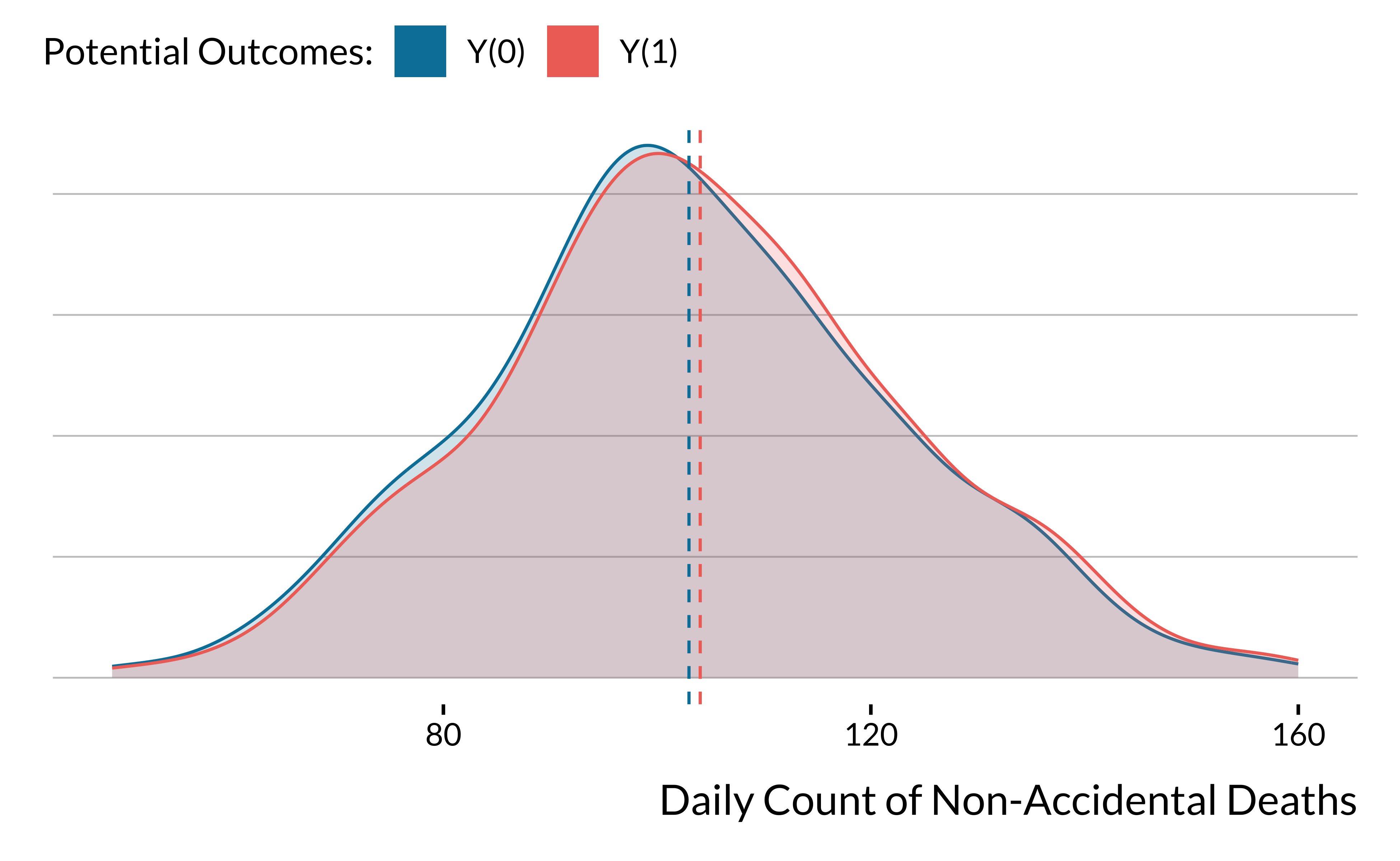
We draw the distribution of non-accidental mortality counts \(Y_i(0)\) from a Negative Binomial distribution with a mean of 106 and a dispersion of 38 (parameter size in the rnbinom function). The variance is equal to \(\simeq\) 402. We choose the parameters to approximate the distribution of non-accidental mortality counts in a major European city.
Our average treatment effect of the air pollutant increase leads to about 1 additional death, which represents a 1% increase in the mean of the outcome. It is a larger effect than what has been found in a very large study based on 625 cities. C. Liu et al. (New England Journal of Medecine, 2019) found that a 10 \(\mu g/m^{3}\) in PM\(_{2.5}\) was associated with an increase of 0.68% (95% CI, 0.59 to 0.77) in daily all-cause mortality.

We display below the Science Table:

And we plot below the full density distribution of the two potential outcomes:

Running the Experiment and Understanding its Inference Properties

In this section, we make the mad scientist run and analyze his experiment. We then show how to think about the inference properties of the experiment when one works in the null hypothesis testing framework.

Running One Iteration of the Experiment

The scientist runs a complete experiment where half of the units are randomly assigned to the treatment. We display below the Science Table and the outcomes observed by the scientists. \(W\) is a binary variable representing the treatment allocation (i.e., it is equal to 1 is the unit is treated and 0 otherwise) and \(Y^{\text{obs}}\) is the potential outcome observed by the scientist given the treatment assignment.

The scientist then estimates the average treatment effect:

Estimate	p-value	95% CI Lower Bound	95% CI Upper Bound
4.16	0.04	0.16	8.17

He obtains an estimate for the treatment effect of 4.16 with a p-value of \(\simeq\) 0.04. “Hooray”, the estimate is statistically significant at the 5% level. The “significant” result fulfills the scientist who immediately starts writing his research paper.

Replicating the Experiment

Unfortunately for the scientist, we are in position where we have much more information than him. We observe the two potential outcomes of each day and we know that the treatment effect is about +1 daily death. To gauge the inference properties of an experiment with this sample size, we replicate 10,000 additional experiments. We use the following function to carry out one iteration of the experiment:

# first add the treatment vector to the science table
data_science_table <- data_science_table %>%
  mutate(w = c(rep(0, n() / 2), rep(1, n() / 2)))

# function to run an experiment
# takes the data as input
function_run_experiment <- function(data) {
  data %>%
    mutate(w = sample(w, replace = FALSE),
           y_obs = w * y_1 + (1 - w) * y_0) %>%
    lm(y_obs ~ w, data = .) %>%
    lmtest::coeftest(., vcov = vcovHC) %>%
    broom::tidy(., conf.int = TRUE) %>%
    filter(term == "w") %>%
    select(estimate, p.value, conf.low, conf.high)
}

We run 10,000 experiments with the code below:

As it takes few minutes, we load the results that we already stored in the data_results_10000_experiments.RDS file in the 1.data folder:

As done by the retrodesign R package, we plot the estimates of all experiments and color them according to the 5% statistical significance threshold:

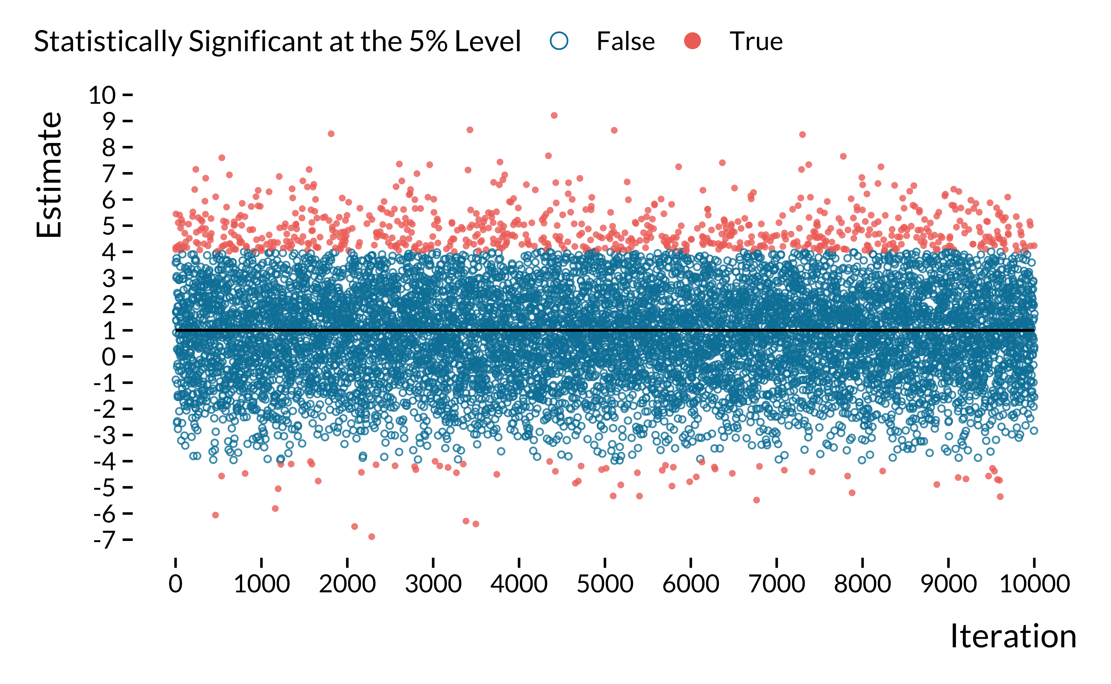
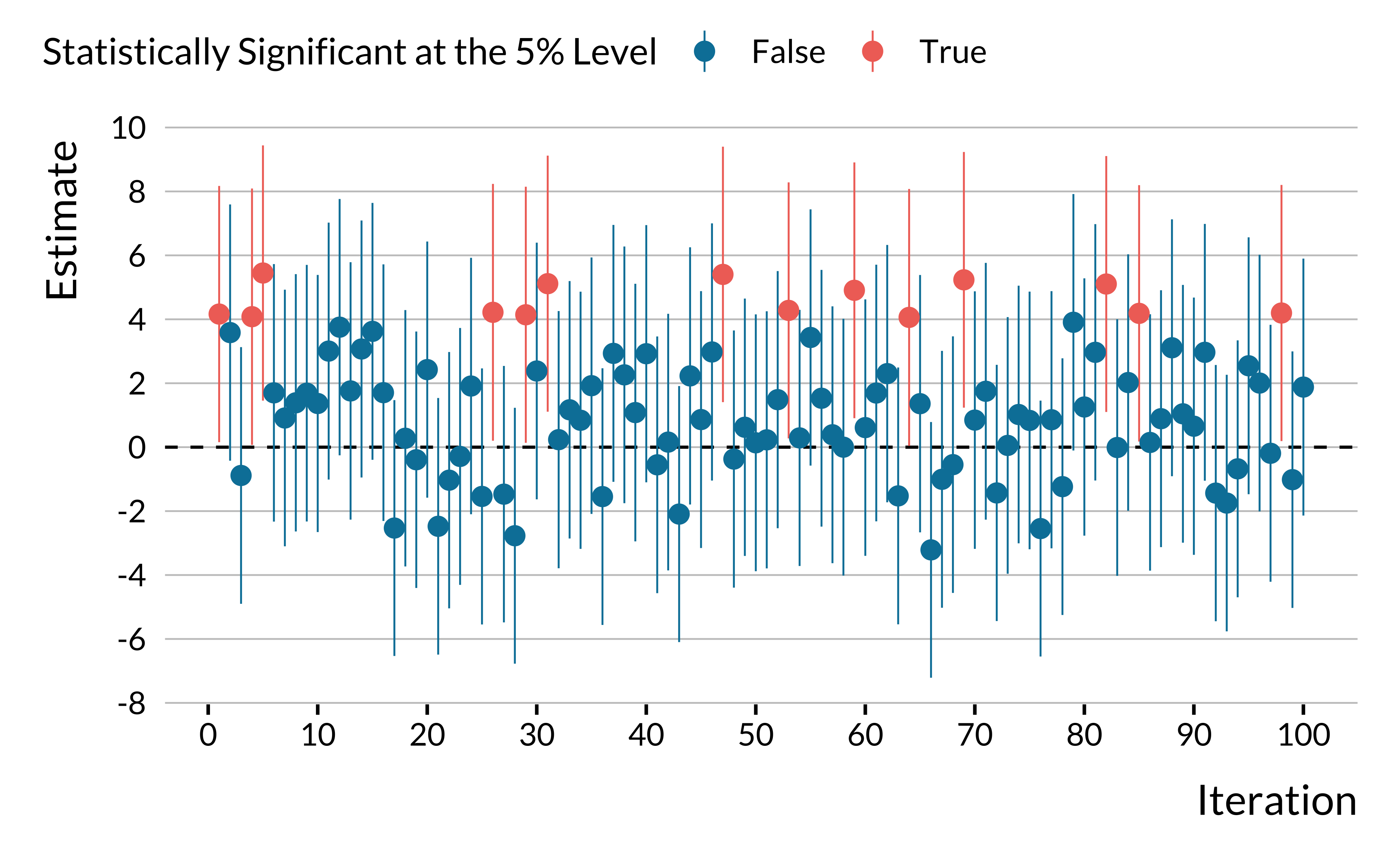
We can see on this graph that statistically significant estimates overestimate the true effect size. Besides, a fraction of significant estimates are of the wrong sign! As an alternative visualization of the replication exercise, we also plot 100 point estimates with their 95% confidence intervals:

Computing Statistical Power, Type M and S Errors

To understand the inference properties of this experiment, we compute three metrics:

The statistical power, which is the probability to get a significant result when there is actually an effect.
The average Type M error, which is the average of the ratio of the absolute value each statistically significant estimate over the true effect size.
The probability to make a Type S error, which is the fraction of statistically significant estimates in the opposite sign of the true effect.

We consider estimates as statistically significant when their associated p-values are inferior or equal to 0.05. First, to compute the statistical power of the experiment, we just need to count the proportion of p-values inferior or equal to 0.05:

The statistical power of this experiment is equal to 8%. The scientist had therefore very few chances to get a “statistically significant” result. We can then look at the characteristics of the statistically significant estimates. We compute the average type M error or exaggeration ratio:

On average, statistically significant estimates exaggerate the true effect size by a factor of about 4.9. We also compute the probability to make a type S error:

Nearly 7.8% of statistically significant estimates are negative! Working with such a sample size to detect an average effect of +1 death could lead to very misleading claims. Finally, we can also check if we could trust confidence intervals of statistically significant effects to capture the true effect size. We compute their coverage rate:

Only 58.1542351% the intervals capture the true effect size! With lower power, the coverage rate of the confidence intervals of statistically significant estimates is much below its expected value of 95%.

How Sample Size Influences Power, Type M and S Errors

Now, imagine that the mad scientist is able to triple the sample of his experiment. We add 732 additional observations:

# set the seed
set.seed(42)

# add extra data
extra_data <-
  tibble(index = c(367:1098),
         y_0 = rnbinom(732, mu = 106, size = 38)) %>%
  mutate(y_1 = y_0 + rpois(n(), mean(y_0) * 1 / 100))

# merge with initial data
data_science_table <- bind_rows(data_science_table, extra_data) %>%
  # add treatment indicator
  mutate(w = c(rep(0, 549), rep(1, 549)))

We run 10,000 experiments for a sample of 1098 daily observations:

As it takes few minutes, we load the results that we have already stored in the data_results_large_sample_experiments.RDS file of the 1.data folder:

We plot the density distribution of the initial and new experiment:

We compute below the statistical power of this larger experiment:

The statistical power of this experiment is equal to 14%. We compute the average type M error:

On average, statistically significant estimates exaggerate the true effect size by a factor of about 3. We also compute the probability to make a type S error:

Nearly 1.9% of statistically significant effects are negative! We finally check the coverage rate of 95% confidence intervals:

The coverage of 95% confidence intervals is equal to 78.2269504%.

With a sample size three times bigger, the statistical power of the experiment has increased but is still very low. Consequently, the exaggeration factor has decreased from 3 to 3. The probability to make a type S error has been reduced a lot and is close to 1. The coverage rate of confidence intervals has increased but is still far from its 95% theoretical target.

Low Statistical Power in the NHST Framework