In this document, we explore the statistical power, type M and S errors of a flagship study by Deryugina et al. (2019) where the authors exploit changes in wind direction to estimate the exogenous effects of PM2.5 on Medicare beneficiaries mortality.
Given a range of hypothetical effect sizes and the standard error displayed in the article, we can compute the statistical power, the exaggeration factor of statistically significant estimate, and the probability that they are of the wrong sign using the retrodesign package. It is a difficult task to evaluate how under-powered a study is as we must guess the true effect size of the variable of interest. We present below different strategies to make informed guesses about the true value of the treatment effect of interest.
Important note: when we give an estimate, we add its associated standard error using the \(\pm\) symbol.
Show the packages used
library("groundhog")
packages <- c(
  "here",
  "tidyverse",
  "knitr",
  "retrodesign",
  "mediocrethemes"
  # "vincentbagilet/mediocrethemes"
)

# groundhog.library(packages, "2022-11-28")
lapply(packages, library, character.only = TRUE)

set_mediocre_all(pal = "leo")
The Mortality and Medical Costs of Air Pollution: Evidence from Changes in Wind Direction
Study Details
Tatyana Deryugina, Garth Heutel, Nolan H. Miller, David Molitor, and Julian Reif (2019) instrument PM\(_{2.5}\) concentrations with wind directions to estimate its effect on mortality, health care use, and medical costs among the US elderly.
Useful details on their study:
- Sample: Their units are daily observations at the county-level over the 1999–2013 period. The sample size is equal to 1 980 549. It is one of the biggest used in the literature.
- First stage: the first stage F-statistic is about 300.
Authors’ main results:
- Using a multivariate linear model, researchers found that that “a 1 microgram per cubic meter (\(\mu g/m^{3}\)) (about 10 percent of the mean) increase in PM 2.5 exposure for one day causes [0.095 \(\pm\) 0.021)] additional deaths per million elderly individuals over the three-day window that spans the day of the increase and the following two days”. In their sample, the three-day mortality rate is 388 per million for individuals aged over 65 years old.
- When instrumented by wind direction, “a 1 microgram per cubic meter (\(\mu g/m^{3}\)) (about 10 percent of the mean) increase in PM 2.5 exposure for one day causes [0.69 \(\pm\) 0.061] additional deaths per million elderly individuals over the three-day window that spans the day of the increase and the following two days”. It represents 0.18% increase in mortality.
Assessing Power, Type M and S Errors
We compute the statistical power, Type M and S errors for alternative and smaller effect sizes than the one found by the authors:
# compute the power, type m and s errors for a range of effect sizes
data_deryugina_2019_iv <-
  retro_design_closed_form(as.list(seq(0.01, 0.7, by = 0.001)), 0.061) %>%
  unnest() %>%
  mutate(power = power * 100, type_s = type_s * 100) %>%
  rename(
    "Statistical Power (%)" = power,
    "Type-S Error (%)" = type_s,
    "Type-M Error (Exaggeration Ratio)" = type_m
  ) %>%
  pivot_longer(
    cols = -c(effect_size),
    names_to = "statistic",
    values_to = "value"
  )
We plot below the power, type M and S errors curves:
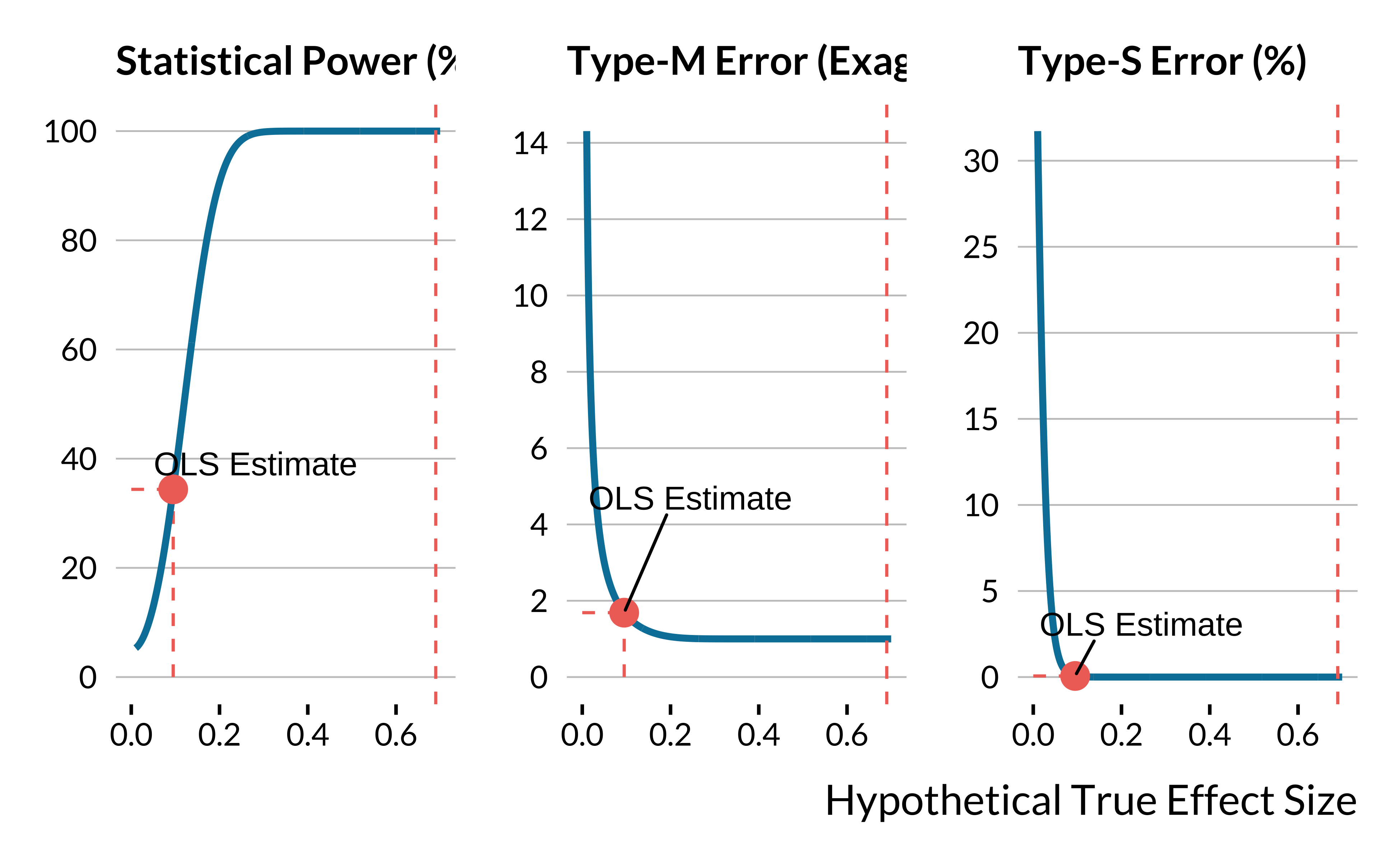
Suppose that the true effect of the increase in PM\(_{2.5}\) was 0.095 additional deaths per million elderly individuals - the estimate found with a naive multivariate model. The statistical power would be 34% and the overestimation factor would be equal to 1.7. The type M error would be worrying for the instrumental variable strategy if the true effect size is the estimate obtained with the standard multivariate model. However, if the true effect size was equal to the lower bound of the 95% confidence interval of the 2SLS estimate, the 1 would be equal to 1: the study would not suffer from a type M error.