Code to load the packages used here
library("groundhog")
packages <- c(
  "here",
  "tidyverse",
  "knitr",
  "patchwork",
  "mediocrethemes"
  # "vincentbagilet/mediocrethemes"
)

# groundhog.library(packages, "2022-11-28")
lapply(packages, library, character.only = TRUE)

set_mediocre_all(pal = "leo")
General Simulations
Loading Data
# load small sample simulation results
summary_evol_large <- readRDS(here("data", "simulations", "summary_evol_large.RDS")) %>%
  mutate(sample_size = "large")

# load large sample simulation results
summary_evol_small <- readRDS(here("data", "simulations", "summary_evol_small.RDS")) %>%
  mutate(sample_size = "small")

# prepare data for graphs
summary_evol_all <- summary_evol_large %>%
  bind_rows(summary_evol_small) %>%
  mutate(
    id_method = case_when(
      id_method == "IV" ~ "Instrumental Variable",
      id_method == "OLS" ~ "Standard Regression",
      id_method == "reduced_form" ~ "Reduced-Form",
      id_method == "RDD" ~ "Discontinuity Design"
    ),
    n_obs = n_days * n_cities
  ) %>%
  pivot_longer(
    cols = c("power", "type_m", "mean_f_stat"),
    names_to = "metrics",
    values_to = "stat_value"
  ) %>%
  mutate(
    metrics_name = case_when(
      metrics == "power" ~ "Statistical Power (%)",
      metrics == "type_m" ~ "Exaggeration Ratio",
      metrics == "mean_f_stat" ~ "F-Statistic",
    ),
    id_method_name = fct_relevel(
      id_method,
      "Standard Regression",
      "Reduced-Form",
      "Instrumental Variable"
    )
  )
Sample Size on Power and Exaggeration
Show code
# make the graph
graph_sample_size <- summary_evol_all  %>%
  filter(id_method != "Discontinuity Design") %>%
  filter(outcome == "death_total") %>%
  filter(percent_effect_size == 1.0) %>%
  filter(p_obs_treat %in% c(NA, 0.5)) %>%
  filter(iv_strength %in% c(NA, 0.5)) %>%
  filter(metrics != "mean_f_stat") %>%
  mutate(n_cities = as.factor(n_cities)) %>%
  ggplot(aes(x = n_days, y = stat_value, colour = n_cities)) +
  geom_line(size = 0.5, linetype = "dashed") +
  geom_point(size = 2.8) +
  facet_grid(fct_rev(metrics_name) ~ id_method_name,
             scale = "free",
             switch = "y") +
  labs(x = "Number of Days",
       y = NULL,
       color = "Number of Cities:") +
  ylim(c(0, NA)) +
  theme(legend.justification = "left")

# print the graph
graph_sample_size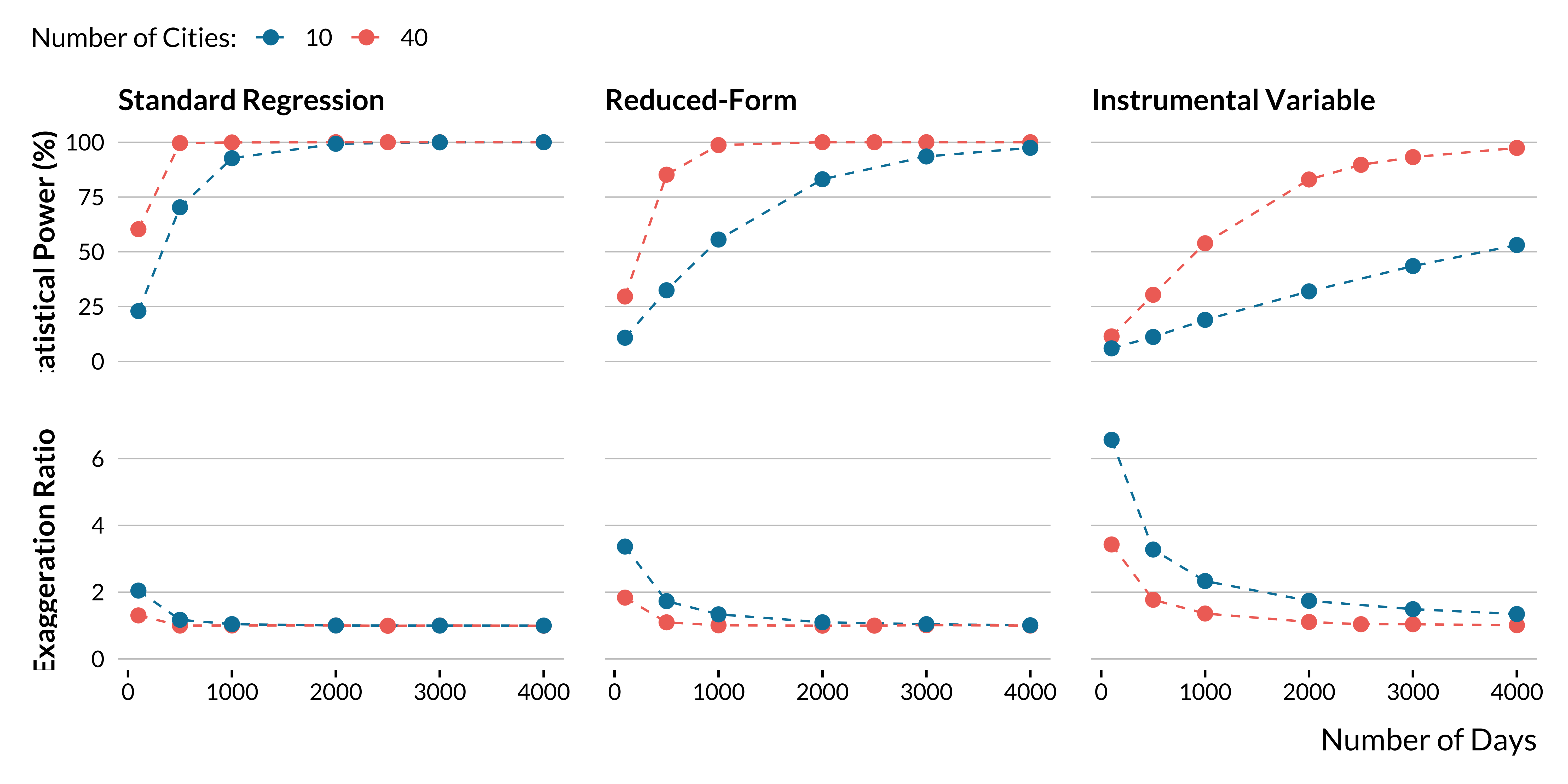
Show code
# save the graph
ggsave(
  graph_sample_size,
  filename = here::here("images", "graph_sample_size.pdf"),
  width = 30,
  height = 20,
  units = "cm"
)
Effect Size on Power and Exaggeration
Show code
# make the graph
graph_effect_size <- summary_evol_all  %>%
  filter(id_method != "Discontinuity Design") %>%
  filter(outcome == "death_total") %>%
  filter(p_obs_treat %in% c(NA, 0.5)) %>%
  filter(iv_strength %in% c(NA, 0.5)) %>%
  filter(metrics != "mean_f_stat") %>%
  filter(n_obs %in% c(10000)) %>%
  ggplot(aes(x = percent_effect_size, y = stat_value)) +
  geom_line(size = 0.5, linetype = "dashed") +
  geom_point(size = 2.8) +
  facet_grid(fct_rev(metrics_name) ~ id_method_name,
             scale = "free",
             switch = "y") +
  labs(x = "Effect Size (%)",
       y = NULL,
       color = "Number of Cities") +
  ylim(c(0, NA))

# print the graph
graph_effect_size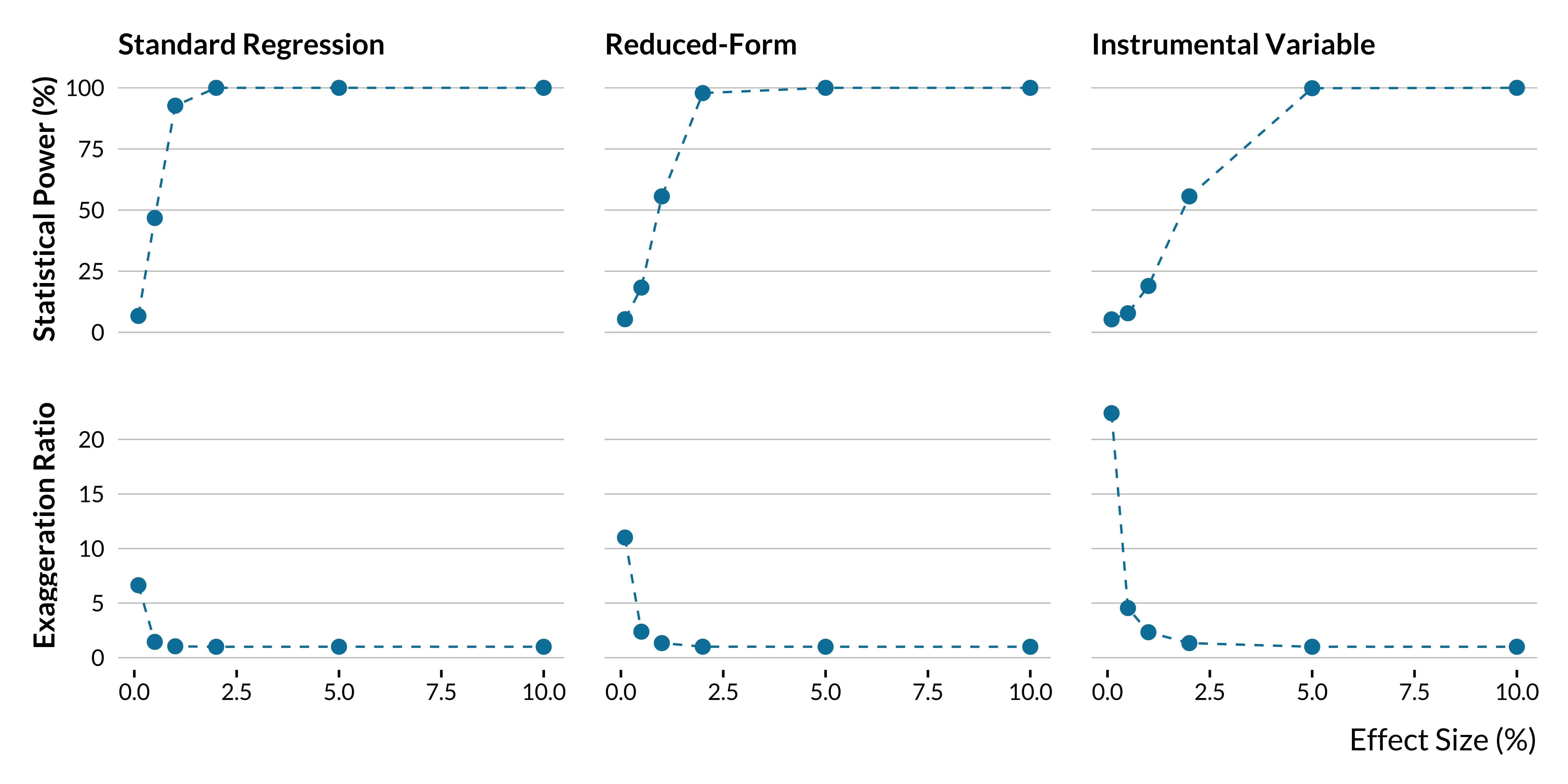
Show code
# save the graph
ggsave(
  graph_effect_size,
  filename = here::here("images", "graph_effect_size.pdf"),
  width = 30,
  height = 20,
  units = "cm"
)
Propotion of Exogenous Shocks on Power and Exaggeration
Show code
# make the graph
graph_prop_exo_shocks <- summary_evol_all %>%
  filter(id_method != "Standard Regression") %>%
  filter(n_obs %in% c(10000, 100000)) %>%
  filter(outcome == "death_total") %>%
  filter(percent_effect_size == 1.0) %>%
  filter(iv_strength %in% c(NA, 0.5)) %>%
  filter(metrics != "mean_f_stat") %>%
  mutate(n_obs = ifelse(n_obs == 10000, "10,000", "100,000")) %>%
  mutate(p_obs_treat = p_obs_treat * 100) %>%
  ggplot(aes(x = p_obs_treat, y = stat_value, colour = n_obs)) +
  geom_line(size = 0.5, linetype = "dashed") +
  geom_point(size = 2.8) +
  facet_grid(fct_rev(metrics_name) ~ id_method_name,
             scales = "free",
             switch = "y") +
  labs(x = "Proportion of Exogenous Shocks (%)",
       y = NULL,
       color = "Sample Size:") +
  ylim(c(0, NA)) +
  theme(legend.justification = "left")

# print the graph
graph_prop_exo_shocks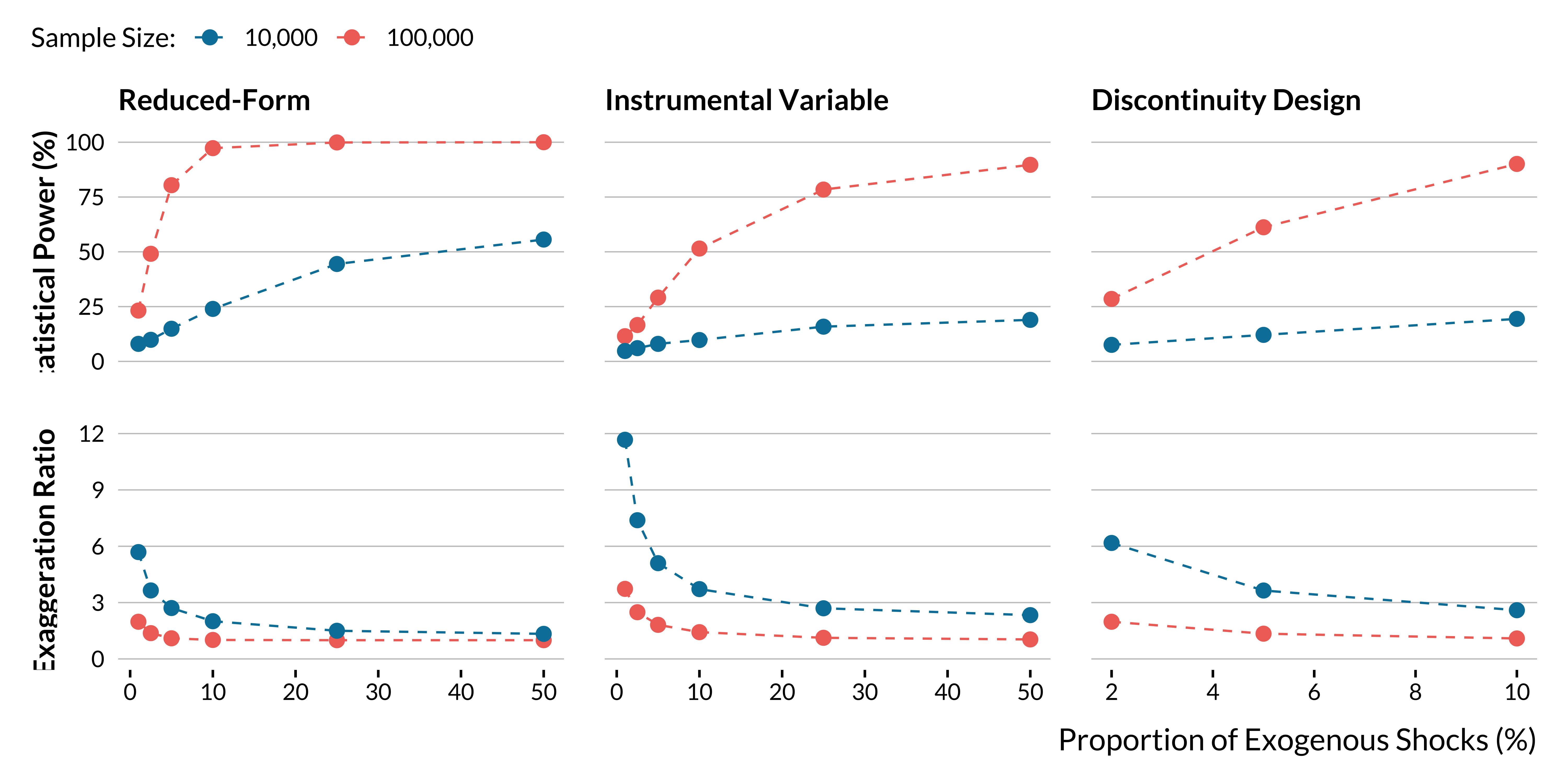
Show code
# save the graph
ggsave(
  graph_prop_exo_shocks,
  filename = here::here("images", "graph_prop_exo_shocks.pdf"),
  width = 30,
  height = 20,
  units = "cm"
)
IV Strength on Power and Exaggeration
Show code
# make the graph
graph_iv <- summary_evol_all %>%
  filter(id_method %in% c("Instrumental Variable")) %>%
  filter(n_days %in% c(1000, 2500)) %>%
  filter(outcome == "death_total") %>%
  filter(percent_effect_size == 1.0) %>%
  filter(p_obs_treat == 0.5) %>%
  mutate(n_cities = as.factor(n_cities)) %>%
  filter(n_obs %in% c(10000, 100000)) %>%
  mutate(n_obs = ifelse(n_obs == 10000, "10,000", "100,000")) %>%
  mutate(metrics_name = fct_relevel(metrics_name, "Statistical Power (%)", "Exaggeration Ratio", "F-Statistic")) %>%
  ggplot(aes(x = iv_strength, y = stat_value, colour = n_obs)) +
  geom_line(size = 0.5, linetype = "dashed") +
  geom_point(size = 2.8) +
  scale_y_continuous(breaks = scales::pretty_breaks(n = 6)) +
  facet_wrap( ~ metrics_name, scale = "free_y") +
  labs(x = "IV First-Stage Effect Size",
       y = NULL,
       color = "Sample Size:")

# print the graph
graph_iv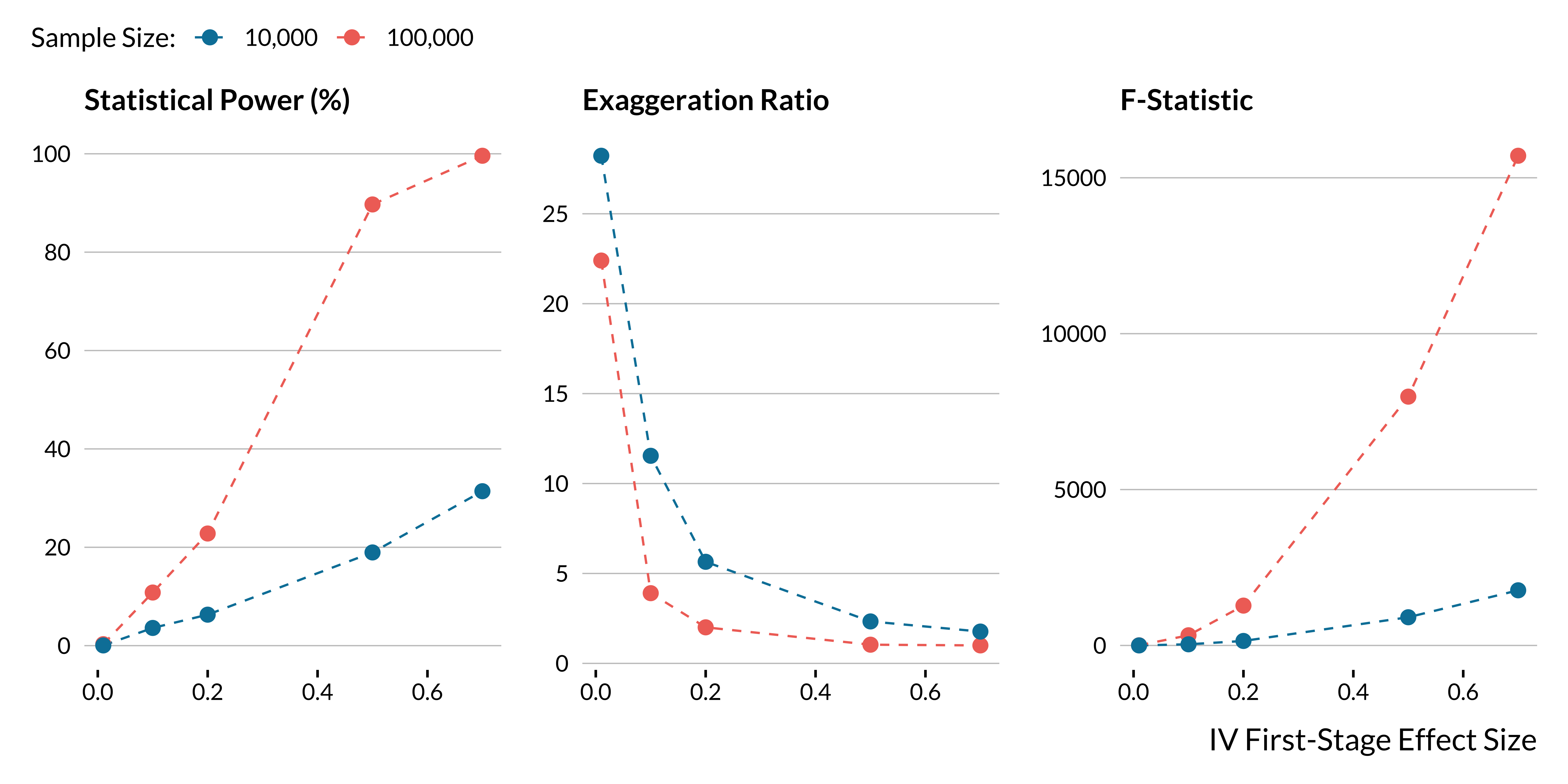
Show code
# save the graph
ggsave(
  graph_iv,
  filename = here::here("images", "graph_iv.pdf"),
  width = 30,
  height = 12,
  units = "cm"
  # device = cairo_pdf
)
Number of cases on Power and Exaggeration
Show code
# make table
summary_evol_all %>%
  filter(id_method %in% c("Instrumental Variable")) %>%
  filter(n_days %in% c(2500)) %>%
  filter(percent_effect_size == 1.0) %>%
  filter(p_obs_treat == 0.5) %>%
  filter(iv_strength == 0.5) %>%
  select(outcome, metrics_name, stat_value) %>%
  pivot_wider(names_from = outcome, values_from = stat_value) %>%
  select(metrics_name, death_total, resp_total, copd_age_65_75) %>%
  mutate_at(vars(-metrics_name), ~ round(., 1)) %>%
  rename(
    "Metric" = metrics_name,
    "Non-Accidental Causes" = death_total,
    "Respiratory Causes" = resp_total,
    "COPD Elderly" = copd_age_65_75
  ) %>%
  knitr::kable(., align = c("l", "c", "c", "c")) %>%
kableExtra::kable_styling(position = "center")| Metric | Non-Accidental Causes | Respiratory Causes | COPD Elderly |
|---|---|---|---|
| Statistical Power (%) | 89.7 | 15.8 | 7.5 |
| Exaggeration Ratio | 1.0 | 2.4 | 5.9 |
| F-Statistic | 7980.3 | 8002.9 | 8045.9 |
Cases Studies
Show code
# modify summarise_simulations to compute mean standard error
summarise_simulations <- function(data) {
  data %>%
    mutate(
      CI_low = estimate + se*qnorm((1-0.95)/2),
      CI_high = estimate - se*qnorm((1-0.95)/2),
      length_CI = abs(CI_high - CI_low),
      covered = (true_effect > CI_low & true_effect < CI_high),
      covered_signif = ifelse(p_value > 0.05, NA, covered) #to consider only significant estimates
    ) %>%
    group_by(formula, quasi_exp, n_days, n_cities, p_obs_treat, percent_effect_size, id_method, iv_strength) %>%
    summarise(
      power = mean(p_value <= 0.05, na.rm = TRUE)*100,
      type_m = mean(ifelse(p_value <= 0.05, abs(estimate/true_effect), NA), na.rm = TRUE),
      type_s = sum(ifelse(p_value <= 0.05, sign(estimate) != sign(true_effect), NA), na.rm = TRUE)/n()*100,
      coverage_rate = mean(covered_signif, na.rm = TRUE)*100,
      coverage_rate_all = mean(covered, na.rm = TRUE)*100,
      mean_se = mean(se, na.rm = TRUE),
      mean_f_stat = mean(f_stat, na.rm = TRUE),
      mean_signal_to_noise = mean(estimate/length_CI, na.rm = TRUE),
      .groups  = "drop"
    ) %>%
    ungroup() %>%
    mutate(
      outcome = str_extract(formula, "^[^\\s~]+(?=\\s?~)"),
      n_days = as.integer(n_days),
      n_cities = as.integer(n_cities)
    )
}
Public Transport Strikes Design
Show code
# load simulations data for reduced form
sim_reduced <-readRDS(here("data", "simulations", "sim_evol_usual_reduced.RDS"))

# get summary of metrics
summary_sim_reduced <- summarise_simulations(sim_reduced)

# check precision
summary_sim_reduced <- summary_sim_reduced %>%
  mutate(
    percentage_precision = case_when(
      outcome == "death_total" ~ mean_se / 23 * 100,
      outcome == "resp_total" ~ mean_se /
        2 * 100,
      outcome == "copd_age_65_75" ~ mean_se /
        0.3 * 100
    )
  )

# function to make a geom_tile graph
function_tiles <- function(data, metric) {
  ggplot(data = data, aes(x = p_obs_treat, y = percent_effect_size, fill = value)) +
    geom_tile(colour = "white", lwd = 2.5, linetype = 1) +
    geom_text(aes(label = round(value, 1)), colour = "black") +
    scale_fill_gradient(name = metric, low = "white", high = "#0081a7") +
    labs(x = NULL, y = NULL) +
    guides(fill = guide_colorbar(title.hjust = 0.5, title.position = "top")) +
    coord_fixed() +
    theme(
      axis.ticks.x = element_blank(),
      axis.ticks.y = element_blank(),
      panel.grid.major.y = element_blank(),
      legend.text=element_text(size=8)
    )
}

# nest the results by metric
nested_summary_sim_reduced <- summary_sim_reduced %>%
  pivot_longer(cols = c(power, type_m, percentage_precision), names_to = "metric", values_to = "value") %>%
  mutate(metric = case_when(metric == "power" ~ "Statistical Power (%)",
                            metric == "type_m" ~ "Exaggeration Factor",
                            metric == "percentage_precision" ~ "Standard Error (%)")) %>%
  mutate(p_obs_treat = p_obs_treat*100) %>%
  mutate_at(vars(p_obs_treat, percent_effect_size), ~ as.factor(.)) %>%
  group_by(metric) %>%
  nest() %>%
  mutate(graph_tile = map2(data, metric, ~ function_tiles(.x, .y)))

# combine the plots
graph_strikes <-
  nested_summary_sim_reduced$graph_tile[[1]] + ylab("Effect Size (%)") + nested_summary_sim_reduced$graph_tile[[2]] + nested_summary_sim_reduced$graph_tile[[3]] + xlab("Proportion of Exogenous Shocks (%)")

# display graph
graph_strikes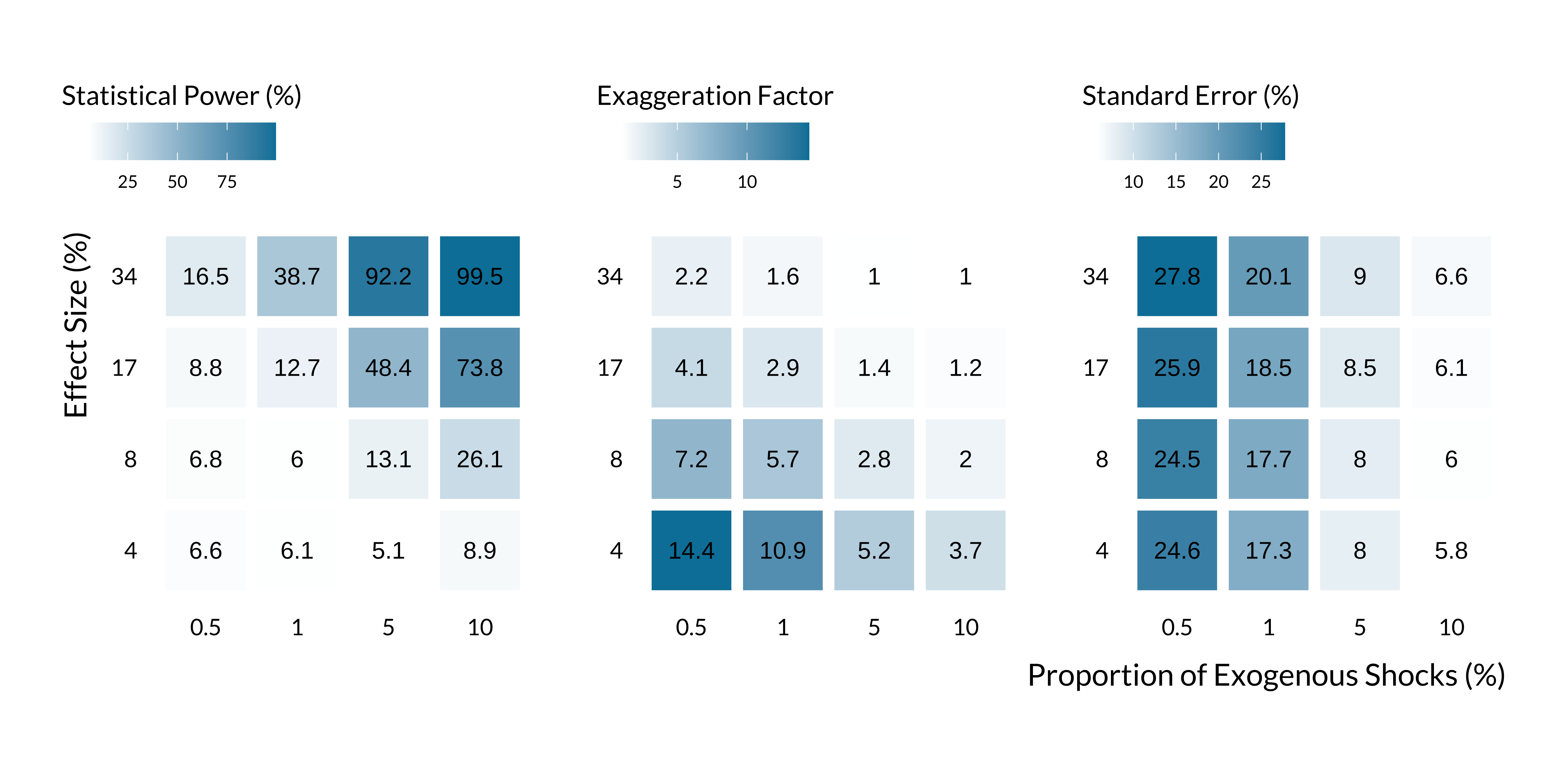
Show code
# save the graph
ggsave(
    graph_strikes,
    filename = here::here("images", "graph_strikes.pdf"),
    width = 30,
    height = 12,
    units = "cm"
    # device = cairo_pdf
  )
Air Pollution Alerts Design
Show code
# load simulations data for reduced form
sim_rdd <- readRDS(here("data", "simulations", "sim_evol_usual_rdd.RDS"))

# get summary of metrics
summary_sim_rdd <- summarise_simulations(sim_rdd)

# check precision
summary_sim_rdd <- summary_sim_rdd %>%
  mutate(
    percentage_precision = case_when(
      outcome == "death_total" ~ mean_se / 23 * 100,
      outcome == "resp_total" ~ mean_se /
        2 * 100,
      outcome == "copd_age_65_75" ~ mean_se /
        0.3 * 100
    )
  )

# function to make a geom_tile graph
function_tiles <- function(data, metric) {
  ggplot(data = data,
         aes(x = p_obs_treat, y = percent_effect_size, fill = value)) +
    geom_tile(colour = "white", lwd = 2.5, linetype = 1) +
    geom_text(aes(label = round(value, 1)), colour = "black") +
    scale_fill_gradient(name = metric, low = "white", high = "#0081a7") +
    labs(x = NULL, y = NULL) +
    guides(fill = guide_colorbar(title.hjust = 0.5, title.position = "top")) +
    coord_fixed() +
    theme(
      axis.ticks.x = element_blank(),
      axis.ticks.y = element_blank(),
      panel.grid.major.y = element_blank(),
      legend.text=element_text(size=8)
    )
}

# nest the results by metric
nested_summary_sim_rdd <- summary_sim_rdd %>%
  pivot_longer(
    cols = c(power, type_m, percentage_precision),
    names_to = "metric",
    values_to = "value"
  ) %>%
  mutate(
    metric = case_when(
      metric == "power" ~ "Statistical Power (%)",
      metric == "type_m" ~ "Exaggeration Factor",
      metric == "percentage_precision" ~ "Standard Error (%)"
    )
  ) %>%
  mutate(p_obs_treat = p_obs_treat * 100) %>%
  mutate_at(vars(p_obs_treat, percent_effect_size), ~ as.factor(.)) %>%
  group_by(metric) %>%
  nest() %>%
  mutate(graph_tile = map2(data, metric, ~ function_tiles(.x, .y)))

# combine the plots
graph_air_quality_alerts <-
  nested_summary_sim_rdd$graph_tile[[1]] + ylab("Effect Size (%)") + nested_summary_sim_rdd$graph_tile[[2]] + nested_summary_sim_rdd$graph_tile[[3]] + xlab("Proportion of Air Quality Alerts (%)")

# display graph
graph_air_quality_alerts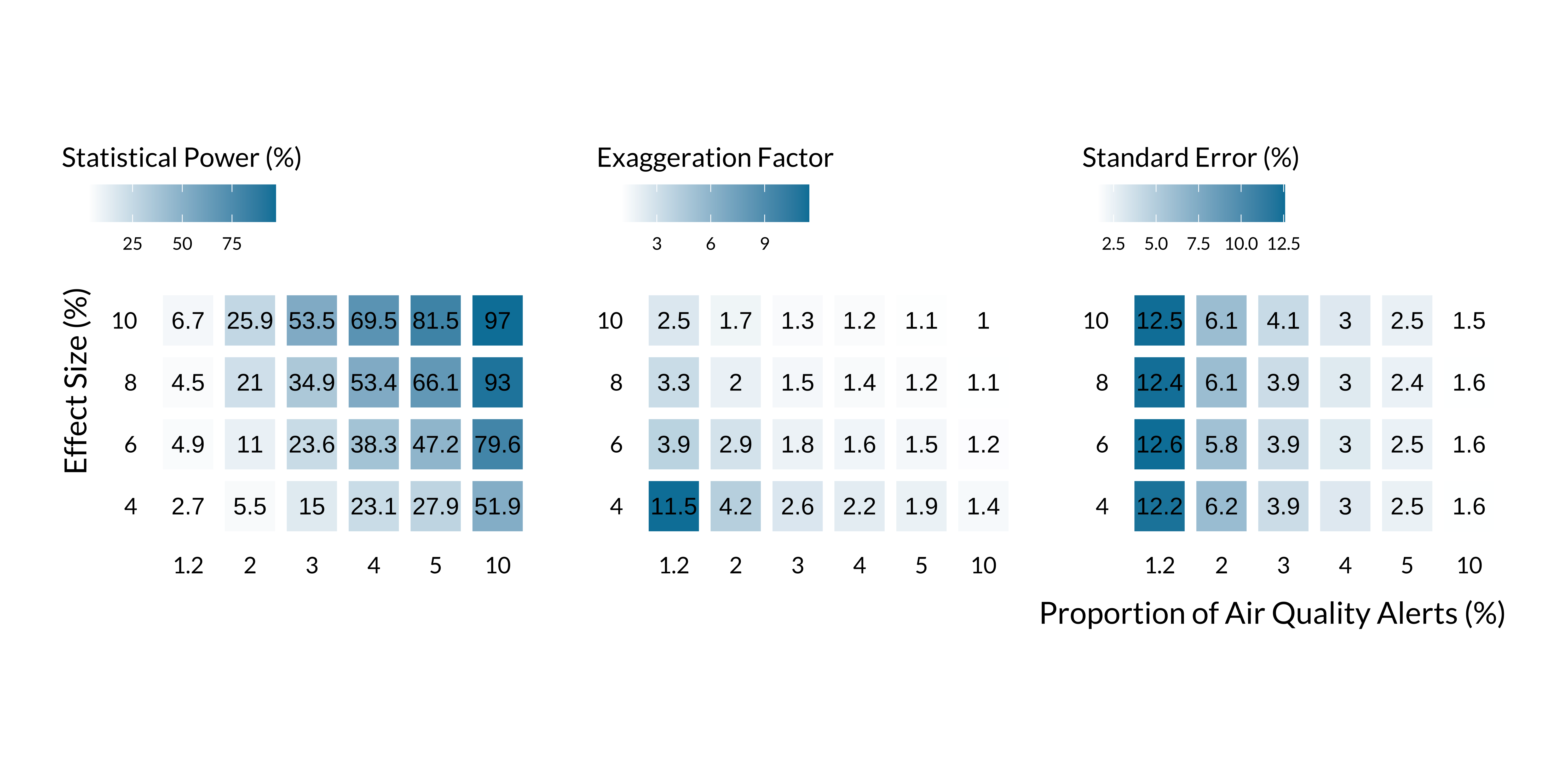
Show code
# save the graph
ggsave(
  graph_air_quality_alerts,
  filename = here::here("images", "graph_air_quality_alerts.pdf"),
  width = 30,
  height = 12,
  units = "cm"
  # device = cairo_pdf
)
Instrumental Variable Design
Show code
# load simulations data for reduced form
sim_iv <- readRDS(here("data", "simulations", "sim_evol_usual_iv.RDS"))

# get summary of metrics
summary_sim_iv <- summarise_simulations(sim_iv)

# check precision
summary_sim_iv <- summary_sim_iv %>%
  mutate(
    percentage_precision = case_when(
      outcome == "death_total" ~ mean_se / 23 * 100,
      outcome == "resp_total" ~ mean_se /
        2 * 100,
      outcome == "copd_age_65_75" ~ mean_se /
        0.3 * 100
    )
  )

# function to make a geom_tile graph
function_tiles <- function(data, metric) {
  ggplot(data = data, aes(x = iv_strength, y = outcome, fill = value)) +
    geom_tile(colour = "white", lwd = 2.5, linetype = 1) +
    geom_text(aes(label = round(value, 1)), colour = "black") +
    scale_fill_gradient(name = metric, low = "white", high = "#0081a7") +
    labs(x = NULL, y = NULL) +
    guides(fill = guide_colorbar(title.hjust = 0.5, title.position = "top")) +
    theme(
      axis.ticks.x = element_blank(),
      axis.ticks.y = element_blank(),
      panel.grid.major.y = element_blank(),
      legend.text=element_text(size=8)
    )
}

# nest the results by metric
nested_summary_sim_iv <- summary_sim_iv %>%
  pivot_longer(cols = c(power, type_m, percentage_precision, mean_f_stat), names_to = "metric", values_to = "value") %>%
  mutate(metric = case_when(metric == "power" ~ "Statistical Power (%)",
                            metric == "type_m" ~ "Exaggeration Factor",
                            metric == "percentage_precision" ~ "Standard Error (%)",
                            metric == "mean_f_stat" ~ "F-Statistic")) %>%
  mutate(outcome = case_when(outcome == "death_total" ~ "Non-Accidental",
                             outcome == "resp_total" ~ "Respiratory",
                             outcome == "copd_age_65_75" ~ "Elderly COPD")) %>%
  mutate(outcome = fct_relevel(outcome, "Elderly COPD", "Respiratory", "Non-Accidental")) %>%
  group_by(metric) %>%
  nest() %>%
  mutate(graph_tile = map2(data, metric, ~ function_tiles(.x, .y)))

# combine the plots
graph_iv_wind <-
  nested_summary_sim_iv$graph_tile[[1]] + nested_summary_sim_iv$graph_tile[[2]] + theme(axis.text.y = element_blank()) + nested_summary_sim_iv$graph_tile[[3]] + nested_summary_sim_iv$graph_tile[[4]] + scale_fill_gradient(name = "F-Statistic", low = "white", high = "#0081a7", breaks = c(2000, 5000, 8000)) + theme(axis.text.y = element_blank()) + xlab("Standardized IV Strength") + plot_layout(ncol = 2)

# display the graph
graph_iv_wind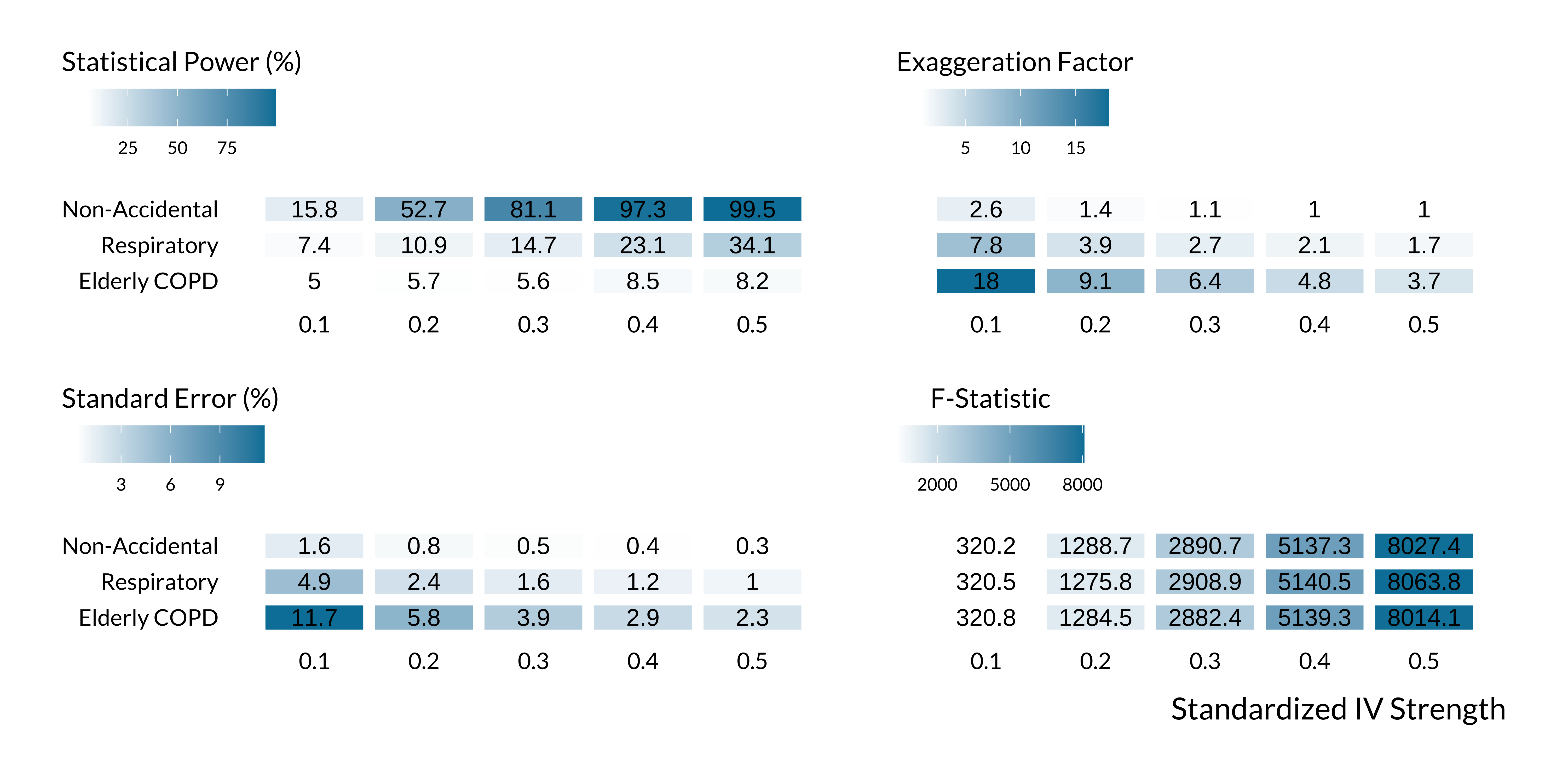
Show code
# save the graph
ggsave(
    graph_iv_wind,
    filename = here::here("images", "graph_iv_wind.pdf"),
    width = 30,
    height = 25,
    units = "cm"
    # device = cairo_pdf
  )