ididvar

The present vignette quickly presents a typical workflow for analysis, using a very basic example. It also provides an overview of most of the functions available in the package.

A more thorough example, with an actual analysis and interpretation of the results, is available on the research project’s website.

Overview of a typical workflow

The workflow to get a better understanding of observations of groups of observations contributing to identification is relatively straightforward:

1. Visualize the relationship between x and y after partialling out (with the idid_viz_bivar function)
2. Compute the observation level weights and add a weight variable to the data set (using idid_weights)
3. Visualize the distribution of these weights (the cumulative with idid_viz_cumul, at the observation and group level with idid_viz_weights or idid_viz_weights_map. To identify groups and variables for which there is a large heterogeneity in weights across groups, use idid_grouping_var). At this stage, one might already get a sense of the effective sample
4. Compute the set of identify contributing observations, ie observations that we can drop without too much altering the estimate (observations whose weight is larger than a threshold computed with idid_contrib_threshold).
5. Visualize contributing observations, both individual and groups (using idid_viz_contrib and idid_viz_contrib_map)
6. Compute and visualize the effective sample size (with idid_viz_drop_change and idid_contrib_stats)

Visualize relationship

Let’s assume we have already ran the regression of interest.

library(ididvar)
library(dplyr)
library(ggplot2)
library(tigris)
library(knitr)

data_ex <- state.x77 |>
  as_tibble() |>
  dplyr::mutate(
    state = rownames(state.x77),
    pop_quartiles = cut_number(Population, 4, labels = FALSE),
    murder_quartiles = cut_number(Murder, 4, labels = FALSE),
    income_quartiles = cut_number(Income, 4, labels = FALSE)
  ) 

reg_ex <-lm(data = data_ex,
            formula = Illiteracy ~  Income + Population + `Life Exp` + Frost)

We first visualize the relationship between x and y (here Illiteracy and Income) after partialling out to understand what we are estimating and to visualize what is driving our

idid_viz_bivar(reg_ex, "Income")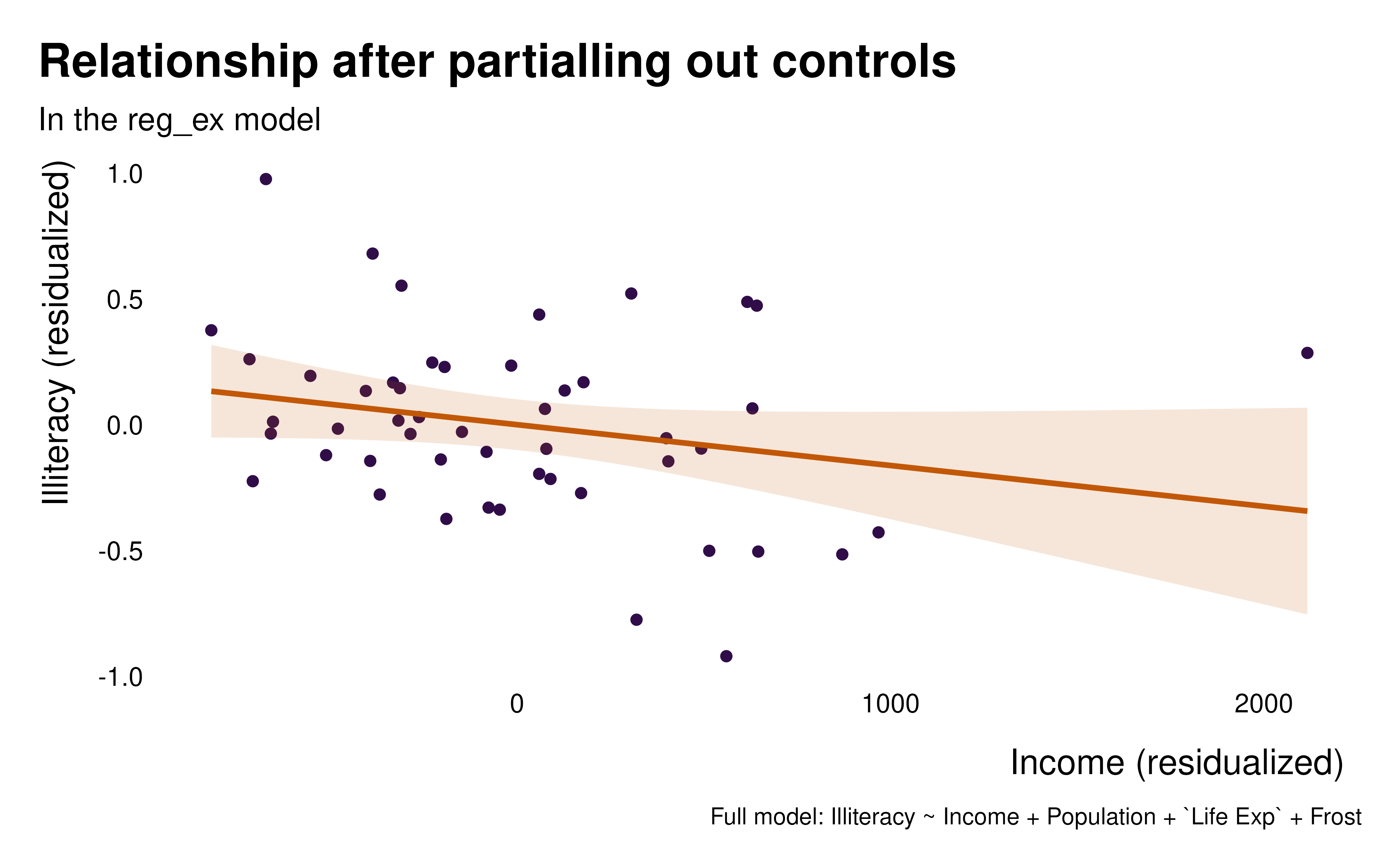

Compute weights

We can add the weights to the data. This step is optional as most functions will recompute the weights.

data_ex_weights <- data_ex |> 
  mutate(idid_weight = idid_weights(reg_ex, "Income"))

Visualize the weights

We can plot the distribution of weights using the idid_viz_cumul function.

idid_viz_cumul(reg_ex, "Income")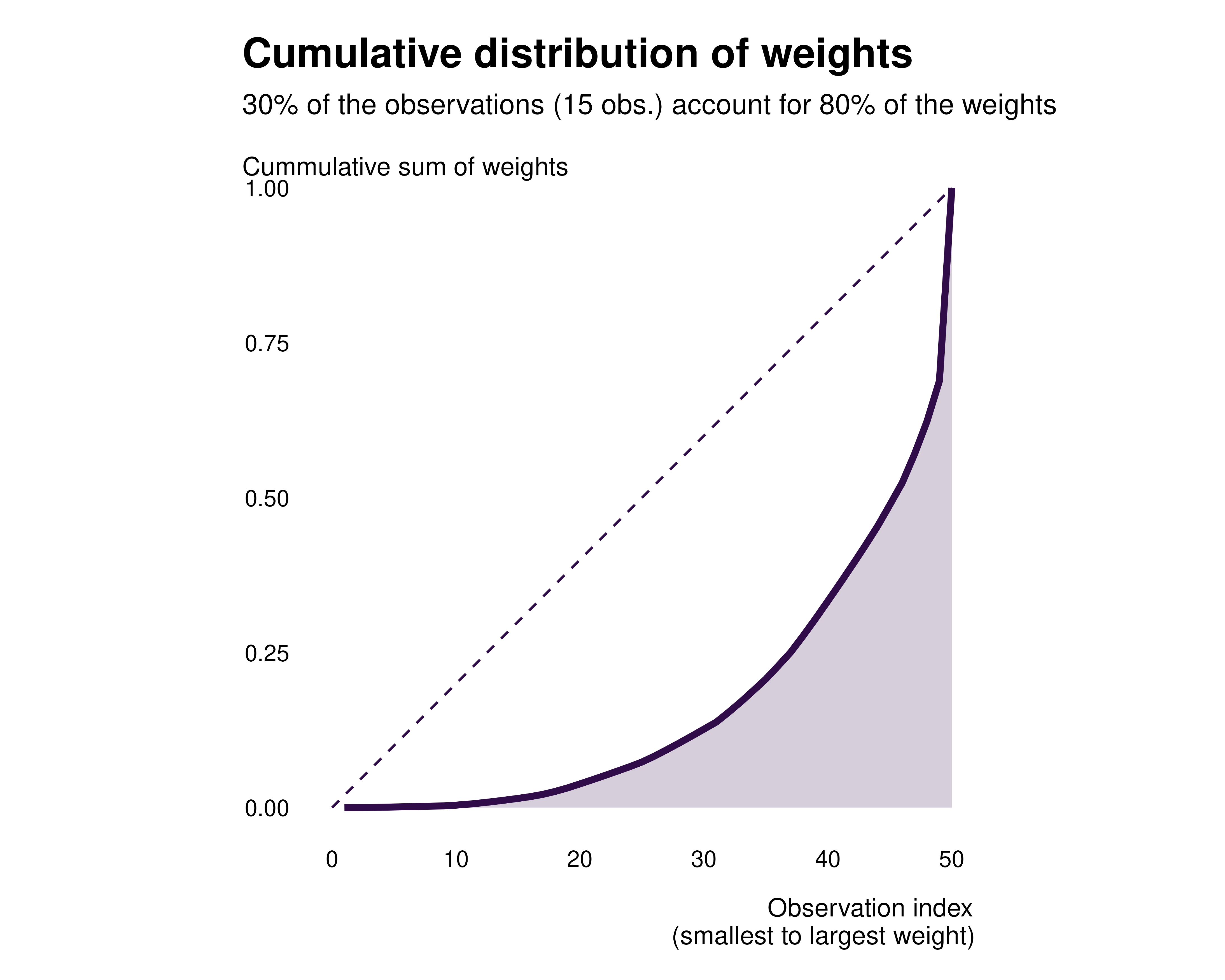

That allows us to analyse the extend to which the weights are evenly distributed. A very unequal distribution should hint that some observations contribute much more to identification and that some observations may not contribute much.

We may then want to explore the distribution of weights, using the idid_viz_weights function. This function makes a graph to visualize the identifying variation weights (a heatmap or a bar chart, depending on the number of dimensions specified). Depending on the shape of the data, there might be some obvious way to analyse it: if, as in the present example, the data is a cross-section, one may want to plot the data by individuals, only providing var_x or var_y to the idid_viz_weights.¹

idid_viz_weights(reg_ex, "Income", var_y = state, order = "y")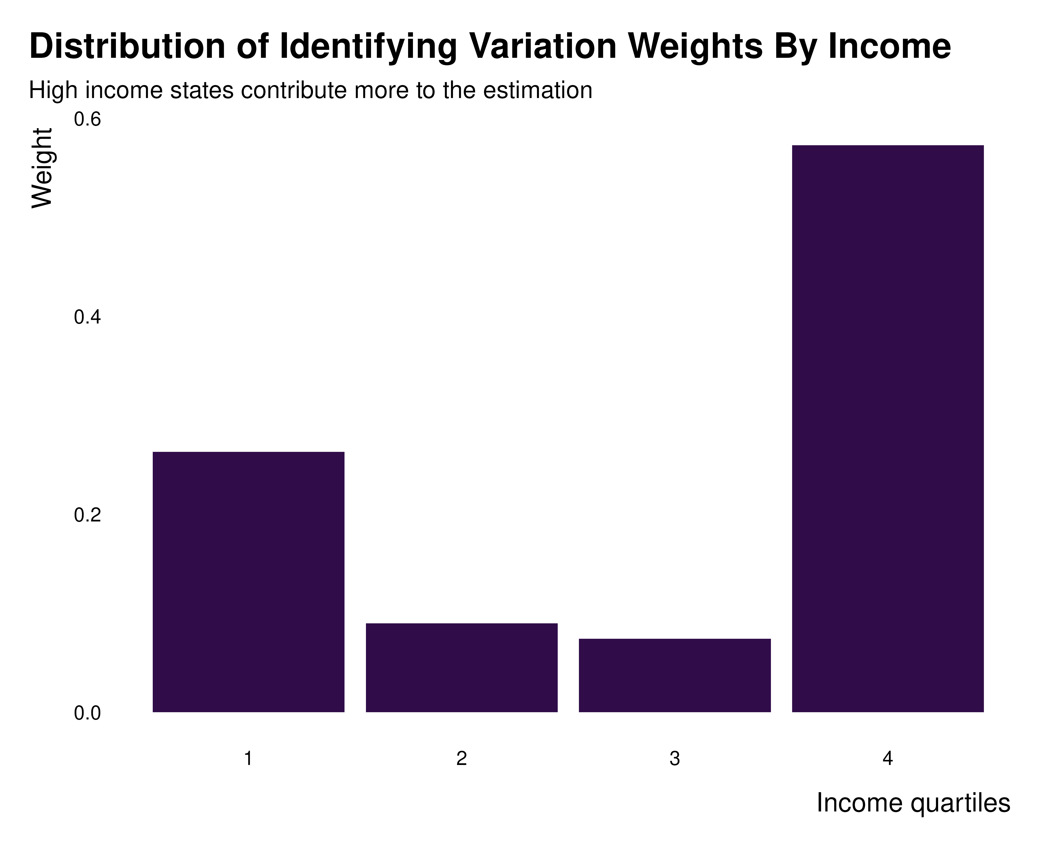

If the data is an individual-time panel, one may want to plot each observation using a heatmap. That can be done with, by providing these two dimensions as the var_x and var_y arguments of idid_viz_weights.

When the data has a geographical dimension, one may want to plot a map of the weights. The function idid_viz_weights_map allows to do easily do that by only providing a shape file in a sf format along with the join variable name.

states_sf <- tigris::states(
    cb = TRUE, resolution = "20m", year = 2024, progress_bar = FALSE) |>
  tigris::shift_geometry() |> 
  rename(state = NAME)

idid_viz_weights_map(reg_ex, "Income", states_sf, "state")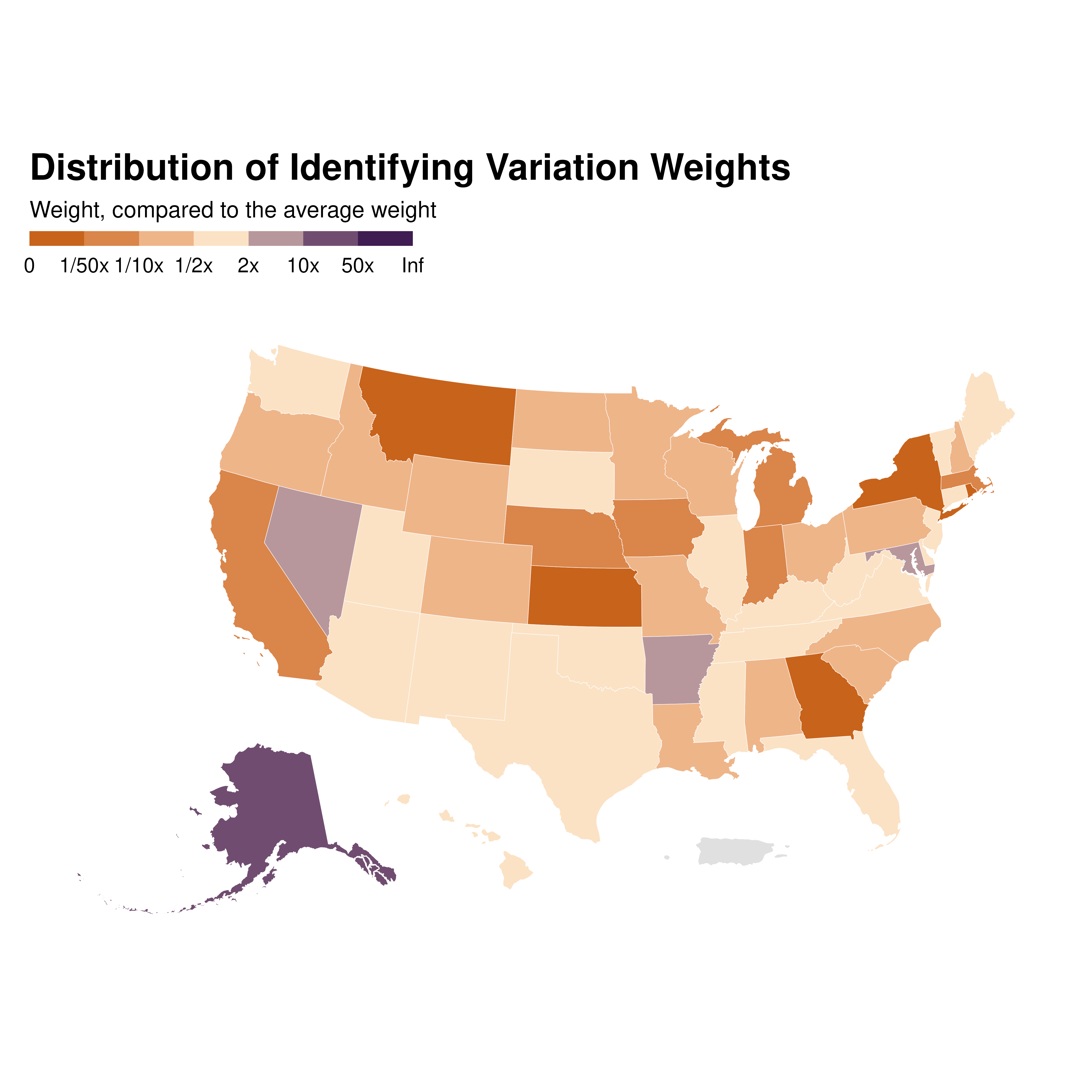

Groups

In addition–or instead–, it is often interesting to analyse whether some groups have larger weights, ie contribute more, than others. One may have a priori ideas regarding which variables to group by. In cases when this might be less clear, one can use idid_grouping_var to identify variables for which groups created by each variable considered (in the grouping_vars argument of the function) have the most between group variance in weights, suggesting a large heterogeneity in weights across groups.

idid_grouping_var(
  reg_ex, "Income", 
  grouping_vars = c("income_quartiles", "pop_quartiles", "murder_quartiles")
) |> 
knitr::kable()

grouping_var	between_var
income_quartiles	0.0536434
pop_quartiles	0.0352604
murder_quartiles	0.0213752

Here, the larges between group variance is across income_quartiles, suggesting that some income group may have larger weights than others. Now that dimensions along which it makes sense to group the weights by have been identify, one can plot the weights distribution across groups.

idid_viz_weights(reg_ex, "Income", income_quartiles) +
  labs(
    x = "Income quartiles", 
    title = "Distribution of Identifying Variation Weights By Income",
    subtitle = "High income states contribute more to the estimation"
  )

Such an analysis can also be implemented for two variables at the same time, thus building heatmaps. This is done with the same method as the one used for individual observations discussed above.

idid_viz_weights(reg_ex, "Income", income_quartiles, pop_quartiles) +
  coord_fixed() +
  labs(x = "Income quartiles", y = "Population quartiles")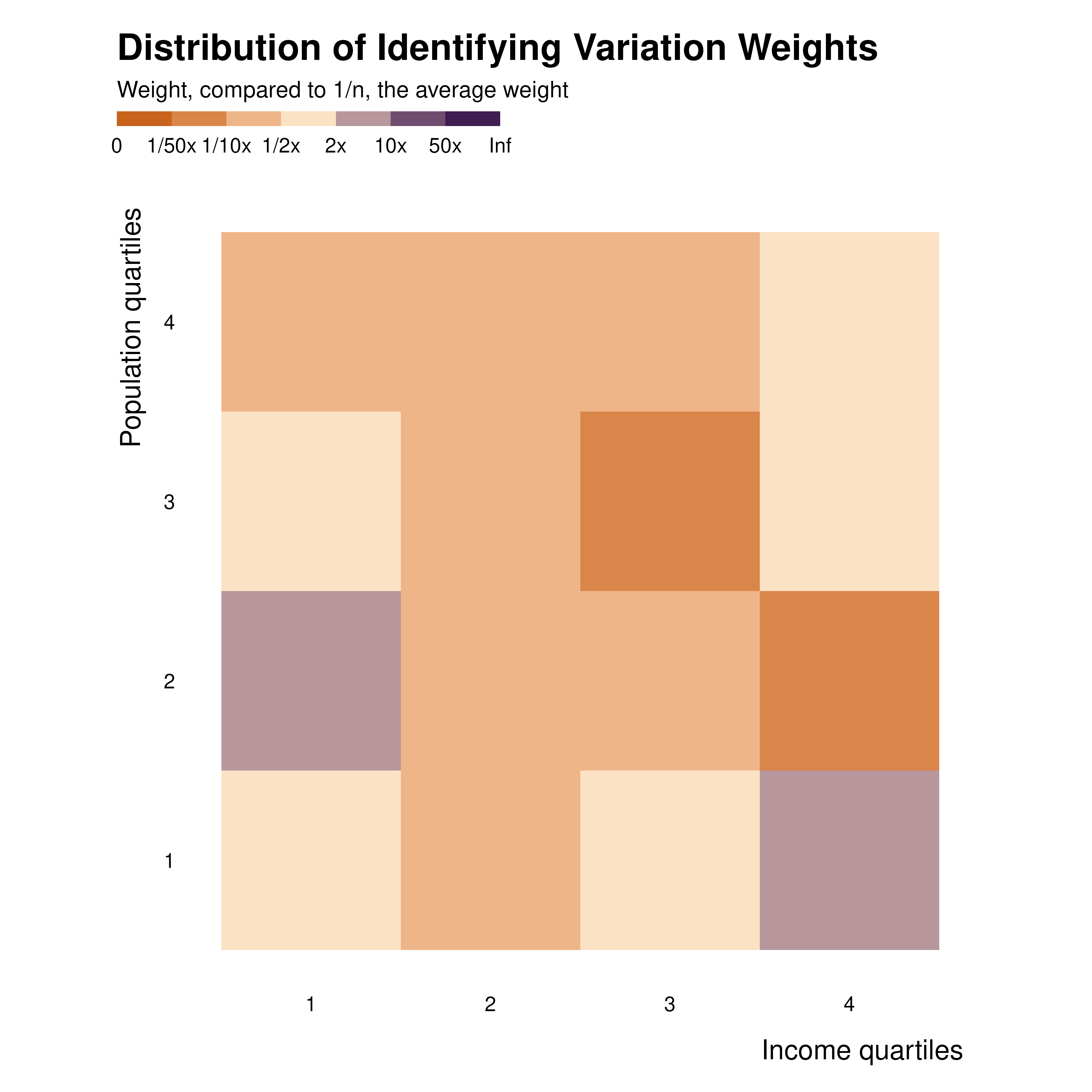

Through all these explorations, one can get a sense of the distribution of weights, through space or groups.

Contribution

We now may wonder which observations contribute to the estimation and which do not. To do so, the present package identifies observations with low weight that can be dropped without affecting the point estimate and standard errors by more than a given proportion.

This can also be illustrated via the idid_viz_drop_change function. It plots a faceted line graph describing the percentage variation of the point estimate and s.e. of interest as a function of the proportion of observations dropped.

idid_viz_drop_change(
  reg_ex, 
  "Income", 
  threshold_change = 0.05, #position of the dotted line
  search_end = 0.4
)

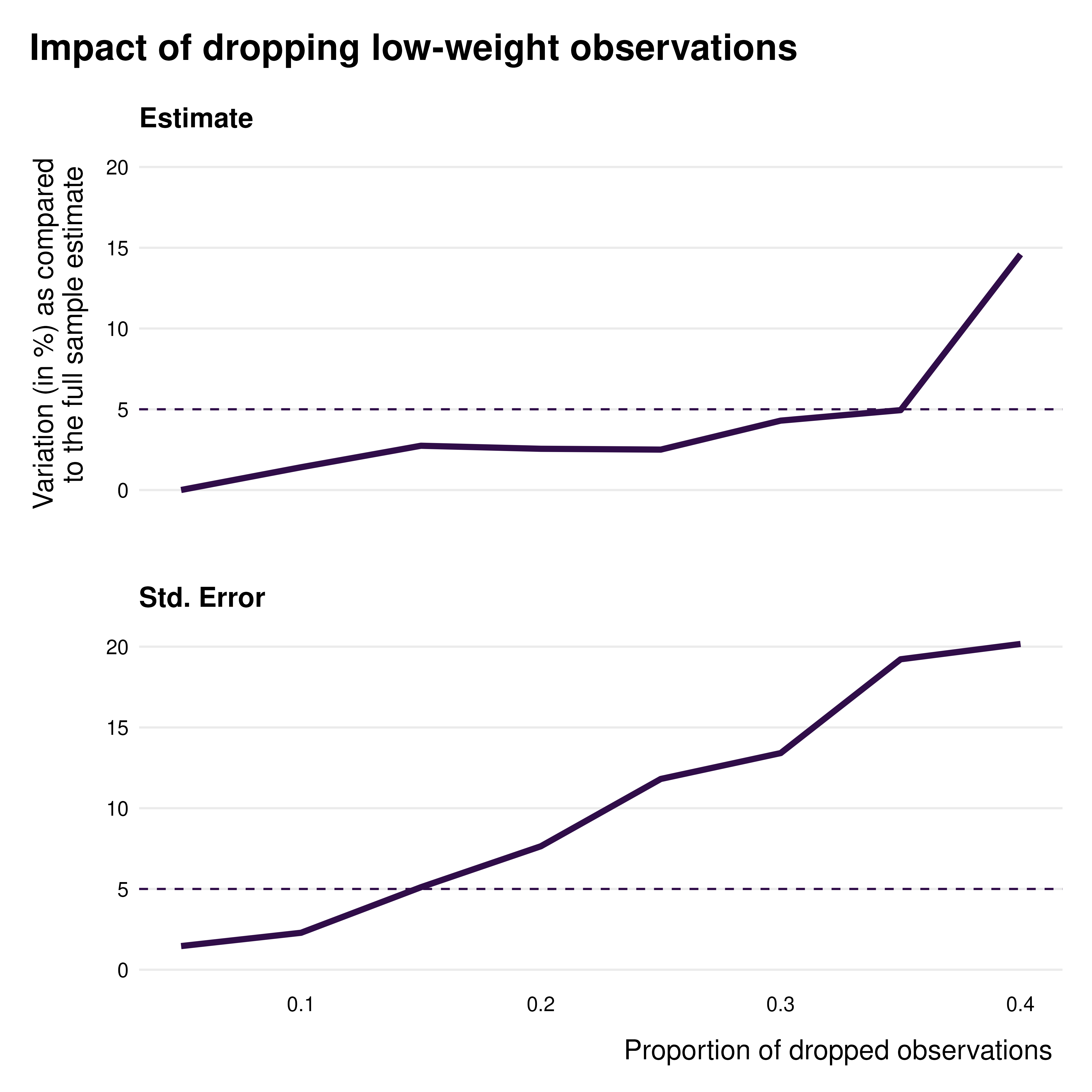
This function loops over the idid_drop_change function which, for a given proportion of observations dropped, computes a variation of the point estimate and standard errors of the coefficient of interest when dropping low weight observations.

Using the idid_contrib_threshold one can identify a weight threshold below which removing observations does not change the point estimate or the standard error of the estimate of interest by more than a given proportion, se 5%:

idid_contrib_threshold(reg_ex, "Income", threshold_change = 0.05)
#> [1] 0.0004276697

All observations with a weight below 4.28^{-4} can be dropped without changing the estimate of interest by more than 5%.

We define the effective sample as the set of observations whose weights are above the aforementioned threshold.

We first use the idid_contrib_stats function to compute the size of this effective sample (as well as of the initial and nominal one):

idid_contrib_stats(reg_ex, "Income") |> 
  knitr::kable()
#> Searching for the contribution threshold

n_initial	n_nominal	n_effective	prop_effective
50	50	43	0.86

We then characterize this effective sample using the idid_viz_contrib and idid_viz_contrib_map functions. They work in a similar ways as idid_viz_weights and idid_viz_weights_map.

idid_viz_contrib(reg_ex, "Income", income_quartiles)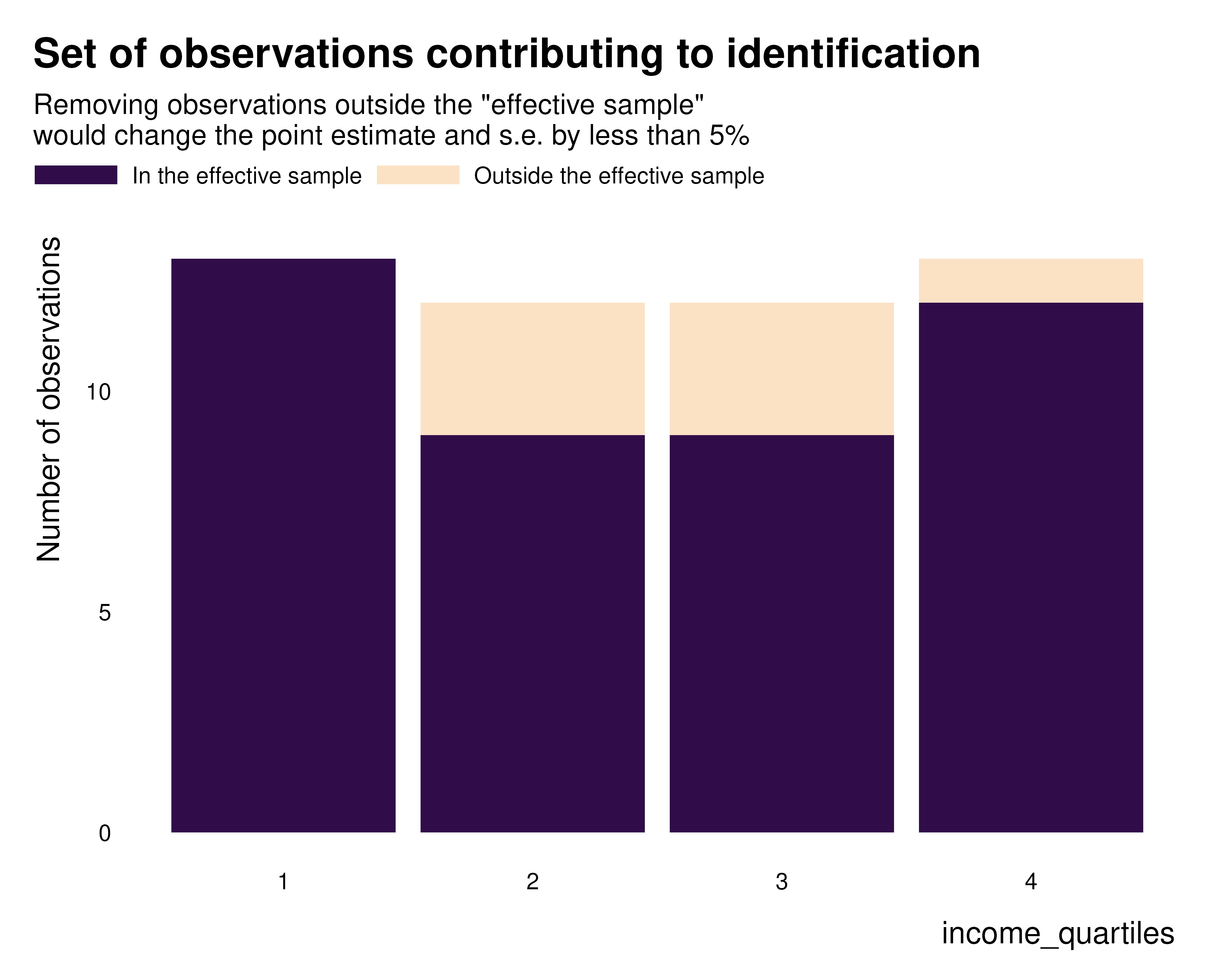
#> Searching for the contribution threshold

idid_viz_contrib_map(reg_ex, "Income", states_sf, "state")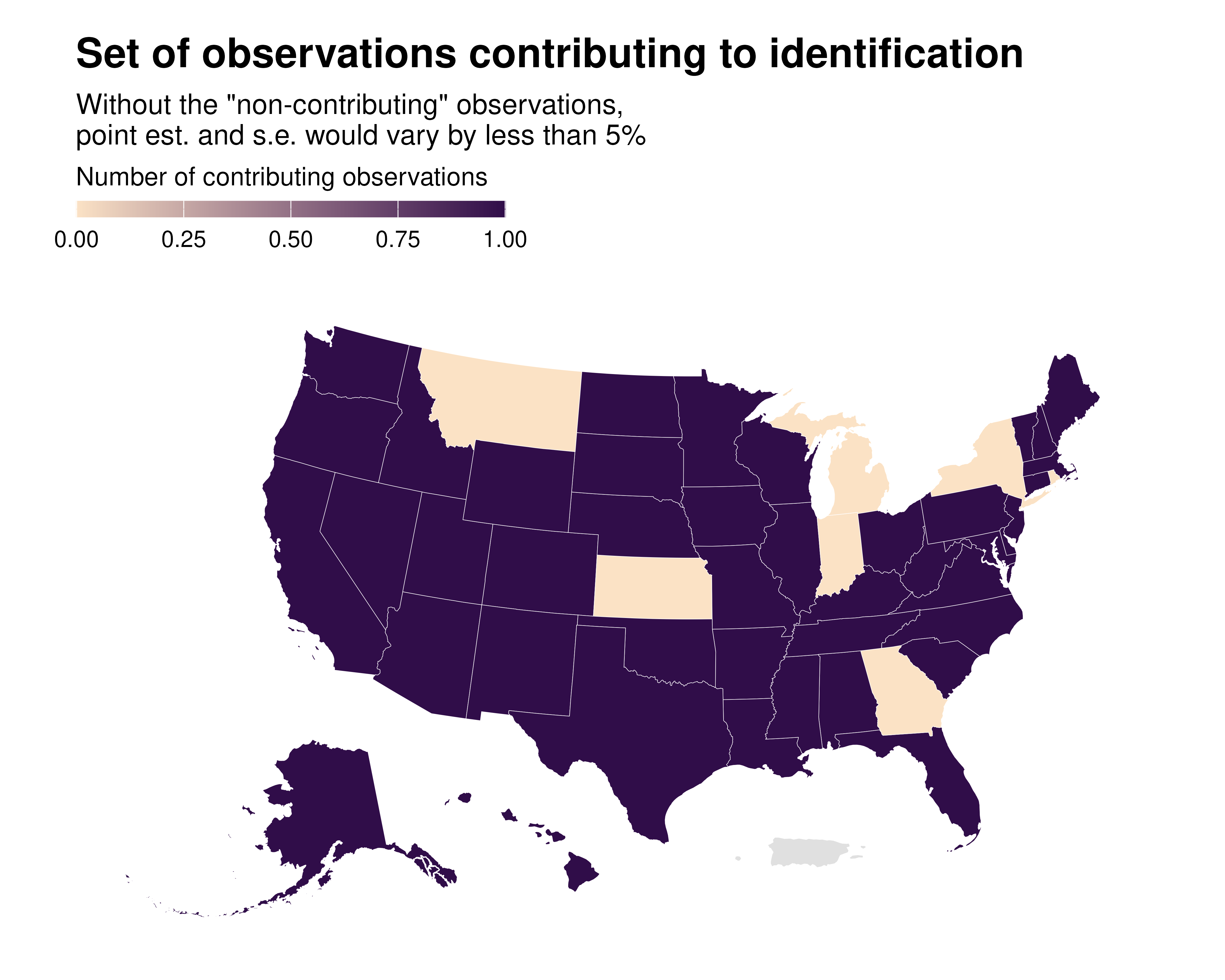
#> Searching for the contribution threshold

Online appendices of the associated paper complements the present vignette by providing an example of a practical implementation of an analysis using the ididvar package.

The “Own visualizations” vignette provides a discussion and code to customize these graphs.