Specification and variation

This document discusses how ididvar can be used to discuss the impact of specification choices on the identifying variation weights and their distribution across observations. In particular, it discusses how the package can provide insights on how different levels of fixed effects affect the weights and the observations contributing to identification.

For this example, let’s use the gapminder data set built on gapminder.org and made available by the gapminder package. It contains data on life expectancy, GDP per-capita and population, for all countries in the world, every 5 years between 1952 and 2007. It is therefore a panel.

library(ididvar)
library(gapminder)
library(fixest)
library(ggplot2)
library(dplyr)
library(purrr)
library(knitr)
library(rnaturalearth)
library(rnaturalearthdata)
library(sf)

In this example, we are interested in studying the relationship between life expectancy and (log-)GDP per capita. We will consider several sets of fixed effects and study their impact on the variation used for identification.

Specifications

Let’s consider 5 regression models: with country, continent, year, continent-year, and country-year fixed effects. We do not include any additional controls for simplicity.

gapminder_ext <- gapminder |> 
  dplyr::mutate(l_gdpPercap = log(gdpPercap)) |> 
  dplyr::filter(continent %in% c("Africa", "Europe")) |>
  dplyr::left_join(gapminder::country_codes, by = join_by(country))

reg_raw <- feols(data = gapminder_ext, lifeExp ~ l_gdpPercap)

reg_continent_fe <- feols(data = gapminder_ext, lifeExp ~ l_gdpPercap | continent, cluster = "continent")

reg_country_fe <- feols(data = gapminder_ext, lifeExp ~ l_gdpPercap | country, cluster = "country")

reg_continent_year_fe <- feols(data = gapminder_ext, lifeExp ~ l_gdpPercap | continent^year, cluster = c("continent^year"))

reg_year_fe <- feols(data = gapminder_ext, lifeExp ~ l_gdpPercap | year, cluster = "year")

reg_twfe <- feols(data = gapminder_ext, lifeExp ~ l_gdpPercap | country + year, cluster = c("country", "year"))

regs <- list(
  reg_raw = reg_raw, 
  reg_continent_fe = reg_continent_fe, 
  reg_country_fe = reg_country_fe, 
  reg_year_fe = reg_year_fe, 
  reg_continent_year_fe = reg_continent_year_fe,
  reg_twfe = reg_twfe
)

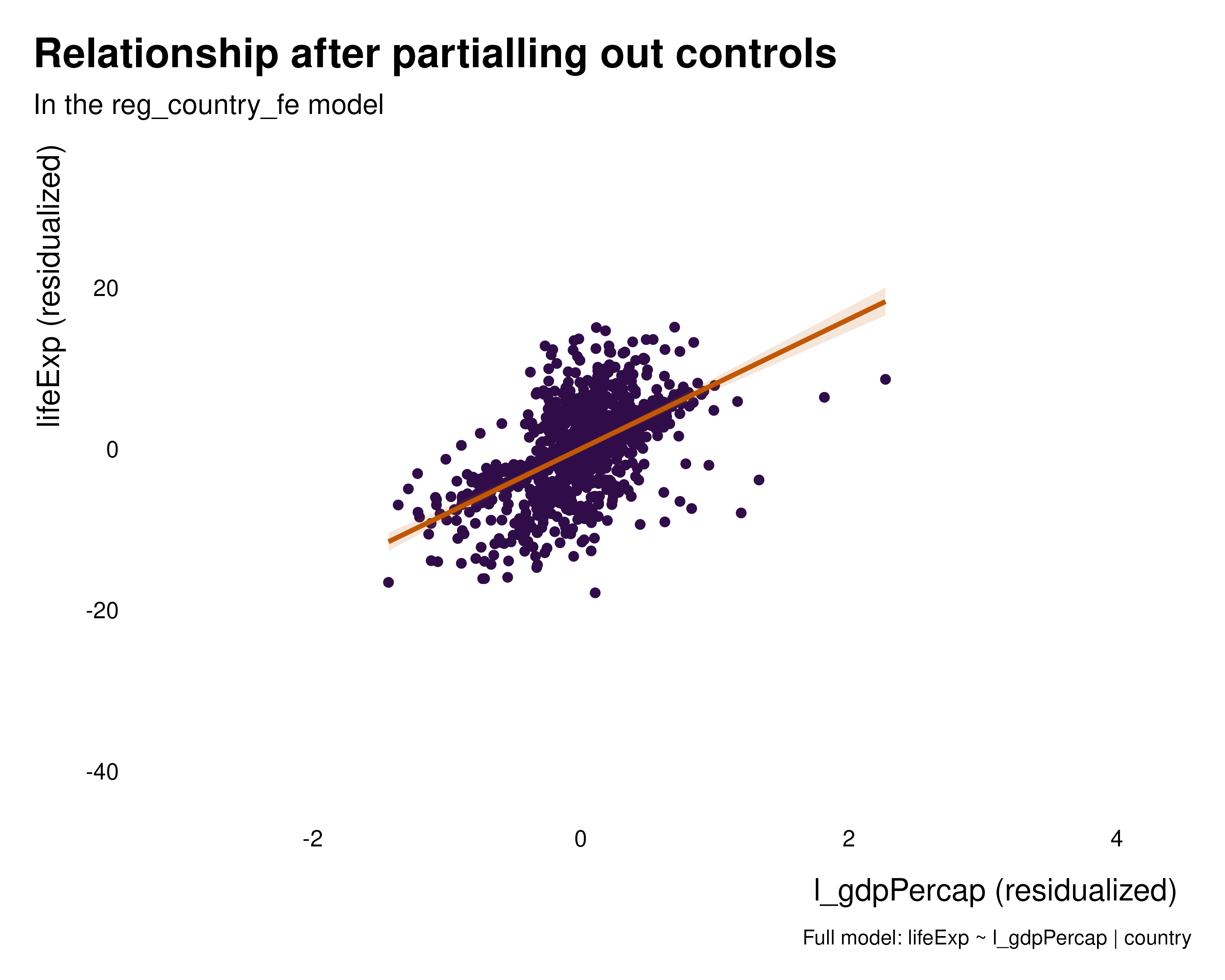
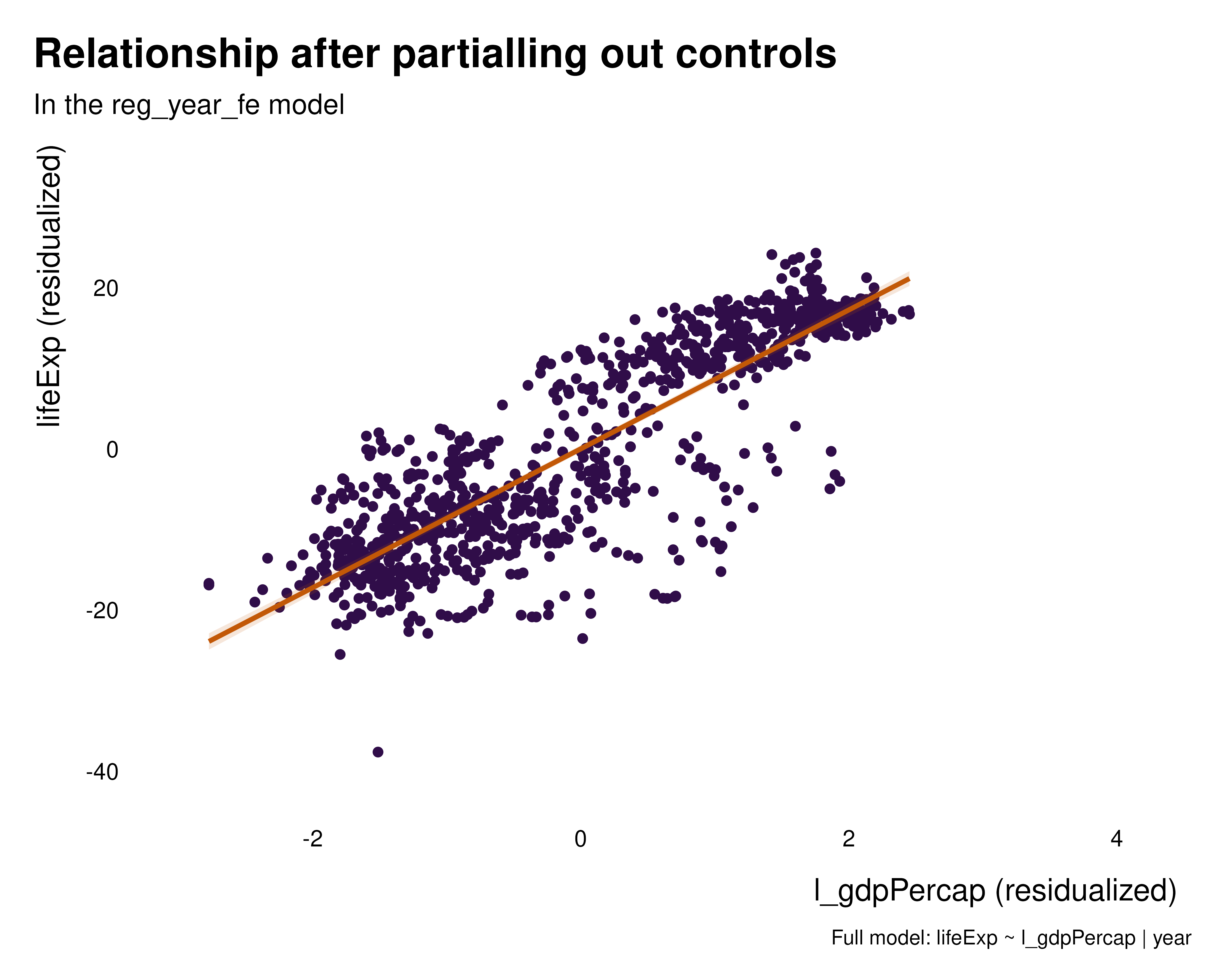
Of course, the parameter on l_gdpPercap does not represent the same quantity in each model. In reg_country_fe, it represents the within country relationship between lifeExp and l_gdpPercap, ie comparing observations at different points in time, within a given country. In reg_year_fe, it represents the within year and therefore across countries.

The goal of this document is to compare across specification the sets of observations that contribute to identification.

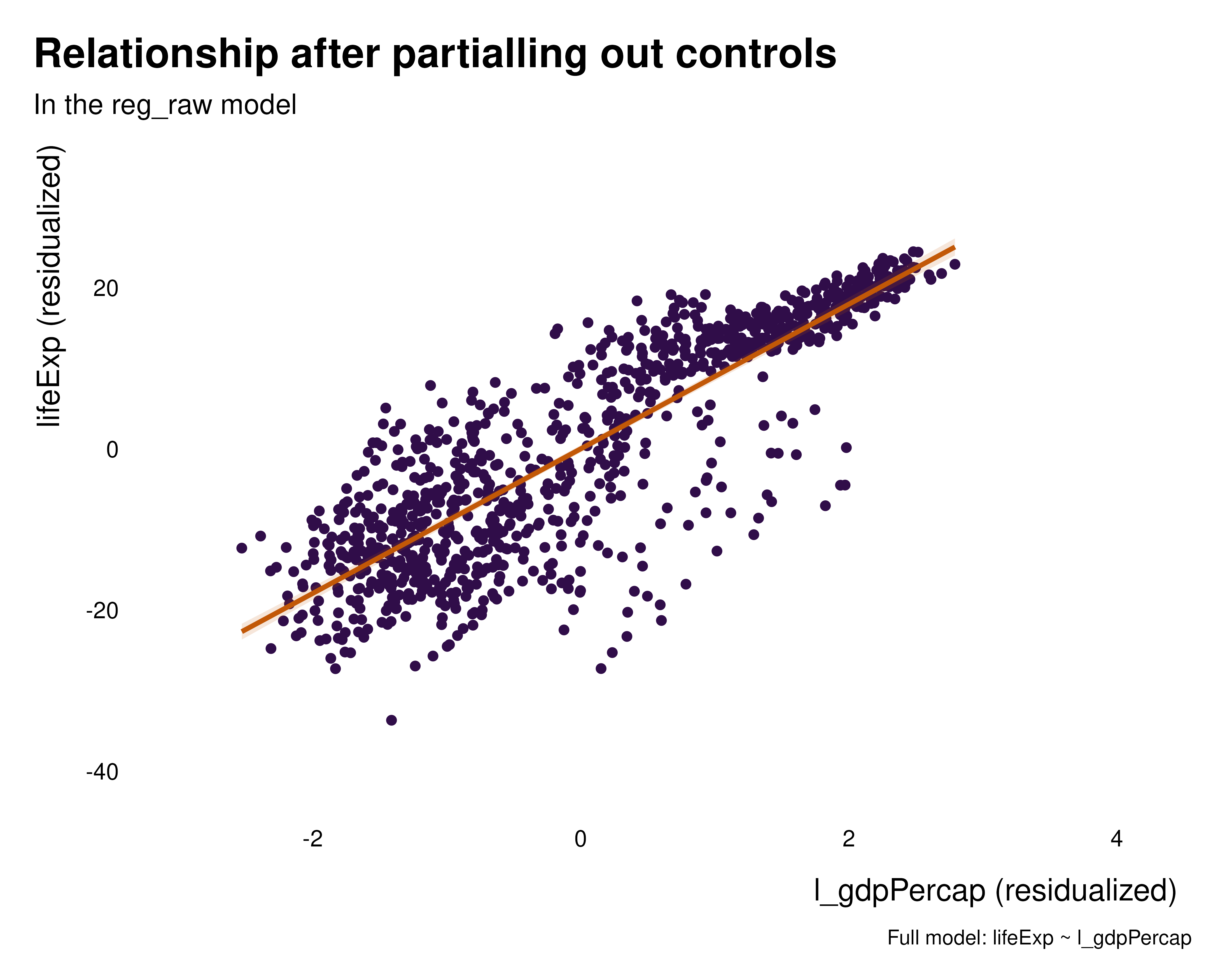
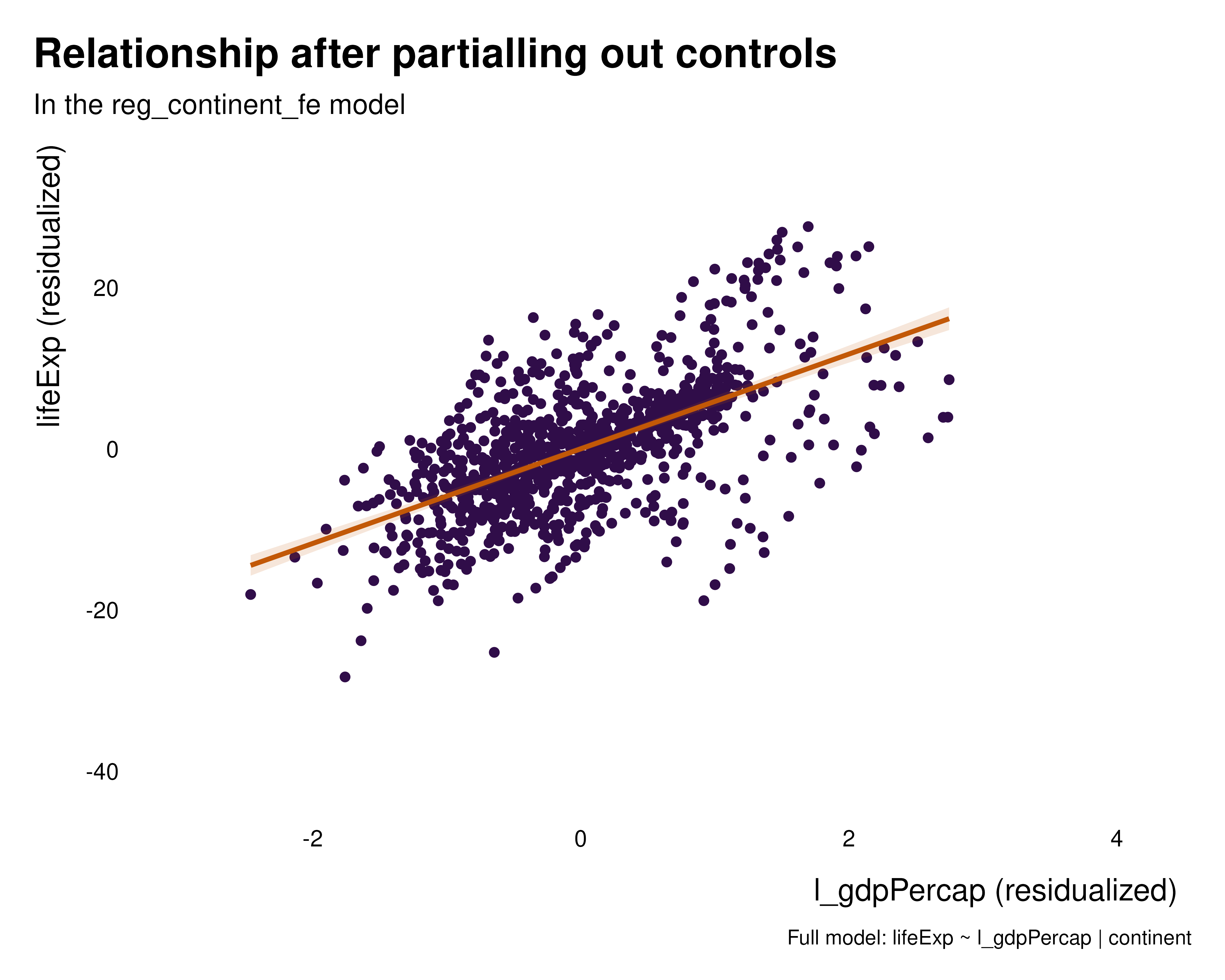
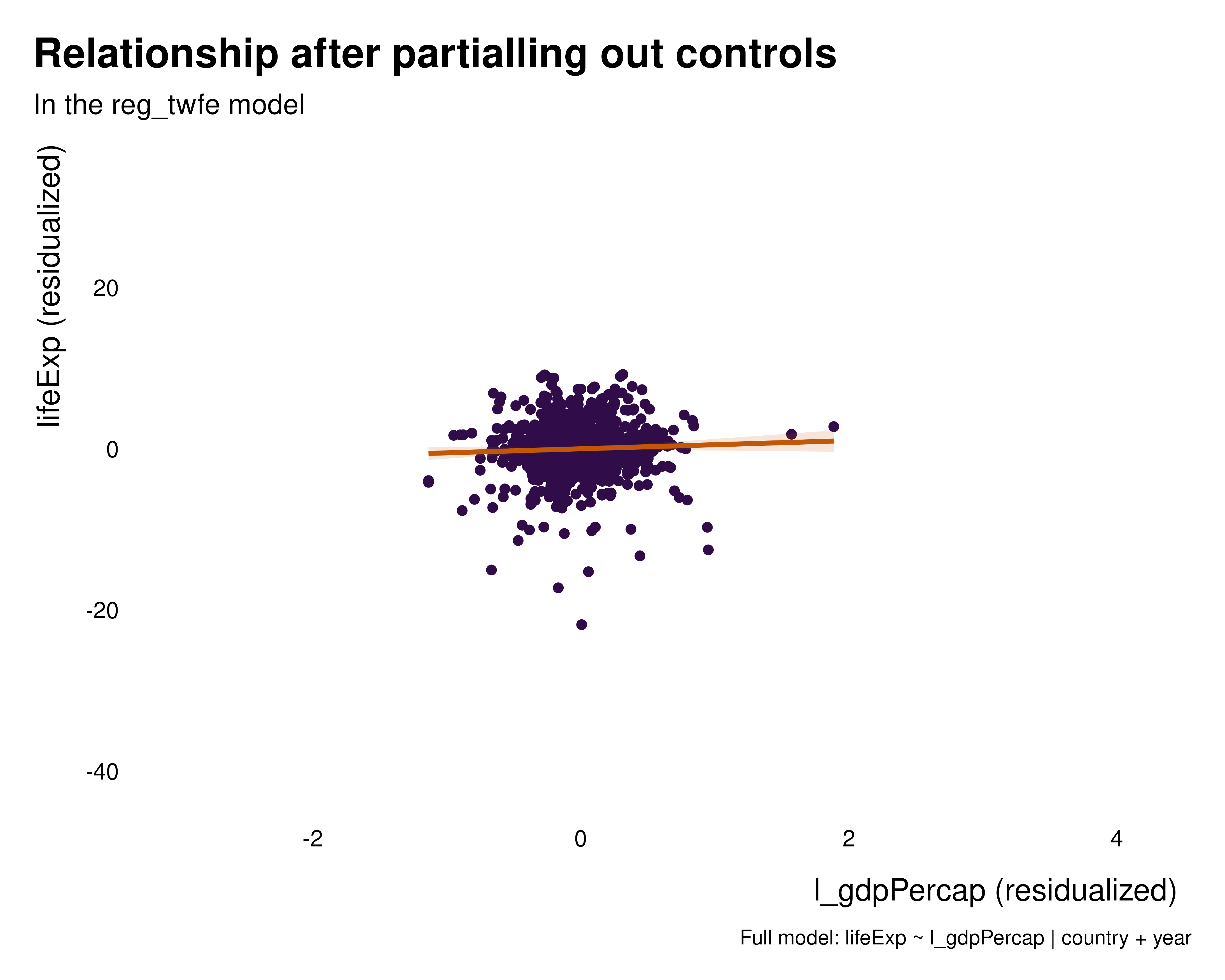
Bivariate graphs

As always in applied econometrics, one the first steps of analysis consists in exploring the raw data and the relationship between the variables of interest.

We can thus plot the partialled out versions of the relationships to get a sense of the variation partialled out by the various sets of fixed effects. These graphs hopefully help understanding what the fixed effects how the fixed effects are affecting the relationship of interest and what variation they are removing. In this particular case, regardless the set of fixed effects, the relationship is positive, despite the quantity estimated being somehow radically different.

• Raw
• Continent FEs
• Country FEs
• Year FEs
• TWFE
• Code

graph_bivar <- function(reg) {
  idid_viz_bivar(reg, "l_gdpPercap") +
    geom_point(aes(color = continent)) +
    lims(x = c(-3, 4.2), y = c(-42, 35)) +
    labs(color = NULL) +
    scale_color_manual(values = c("#497C89", "#cf816b"))
}

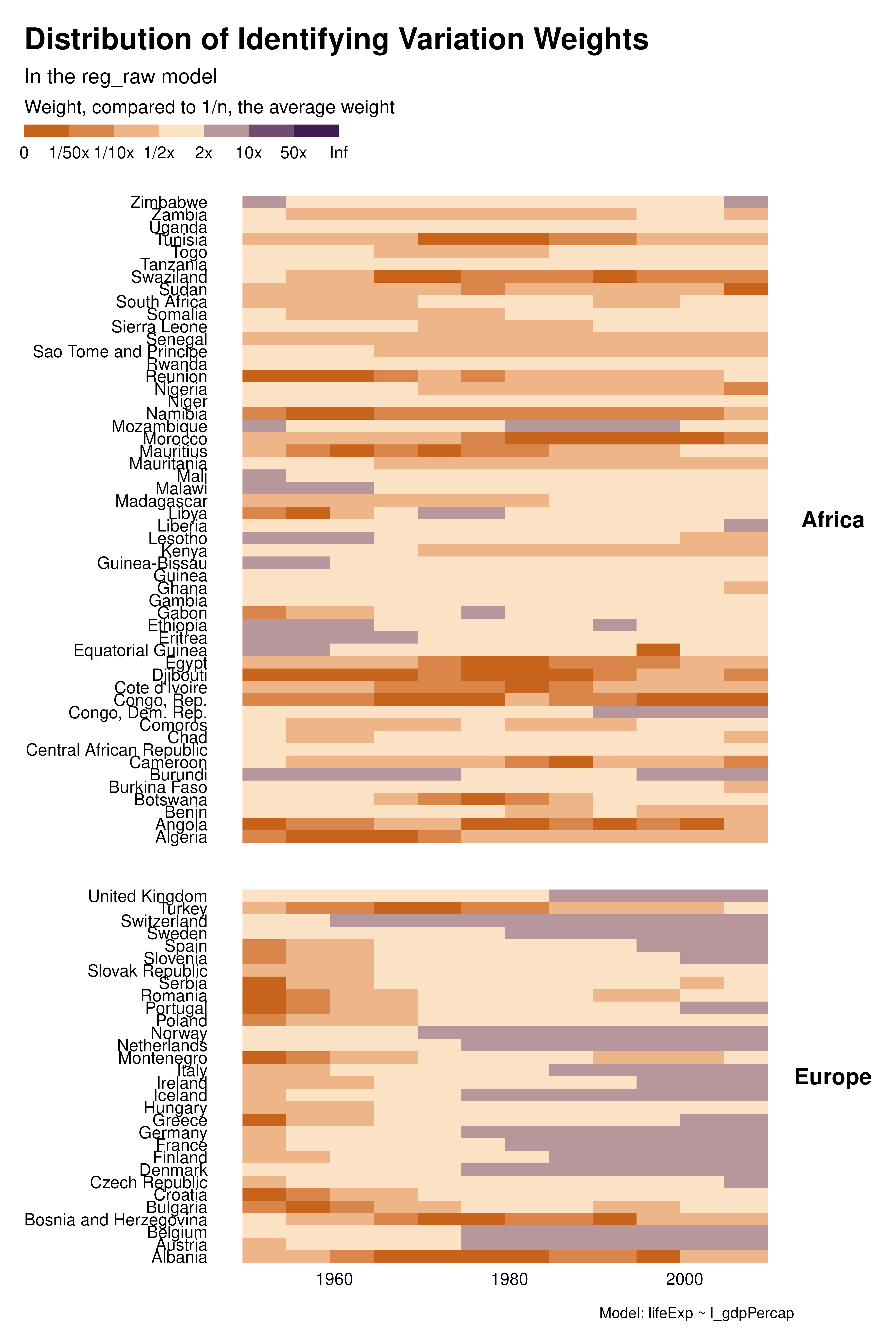
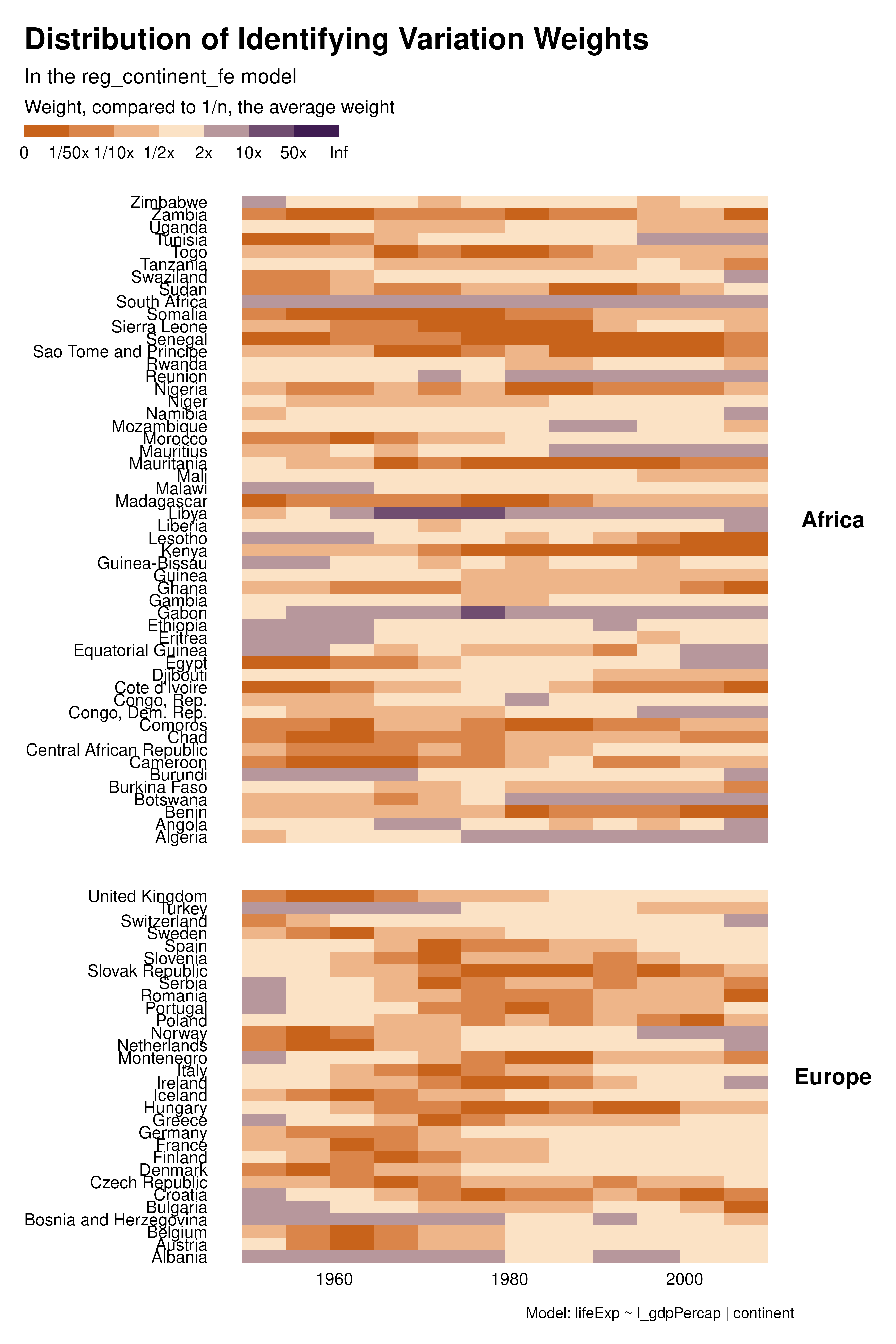
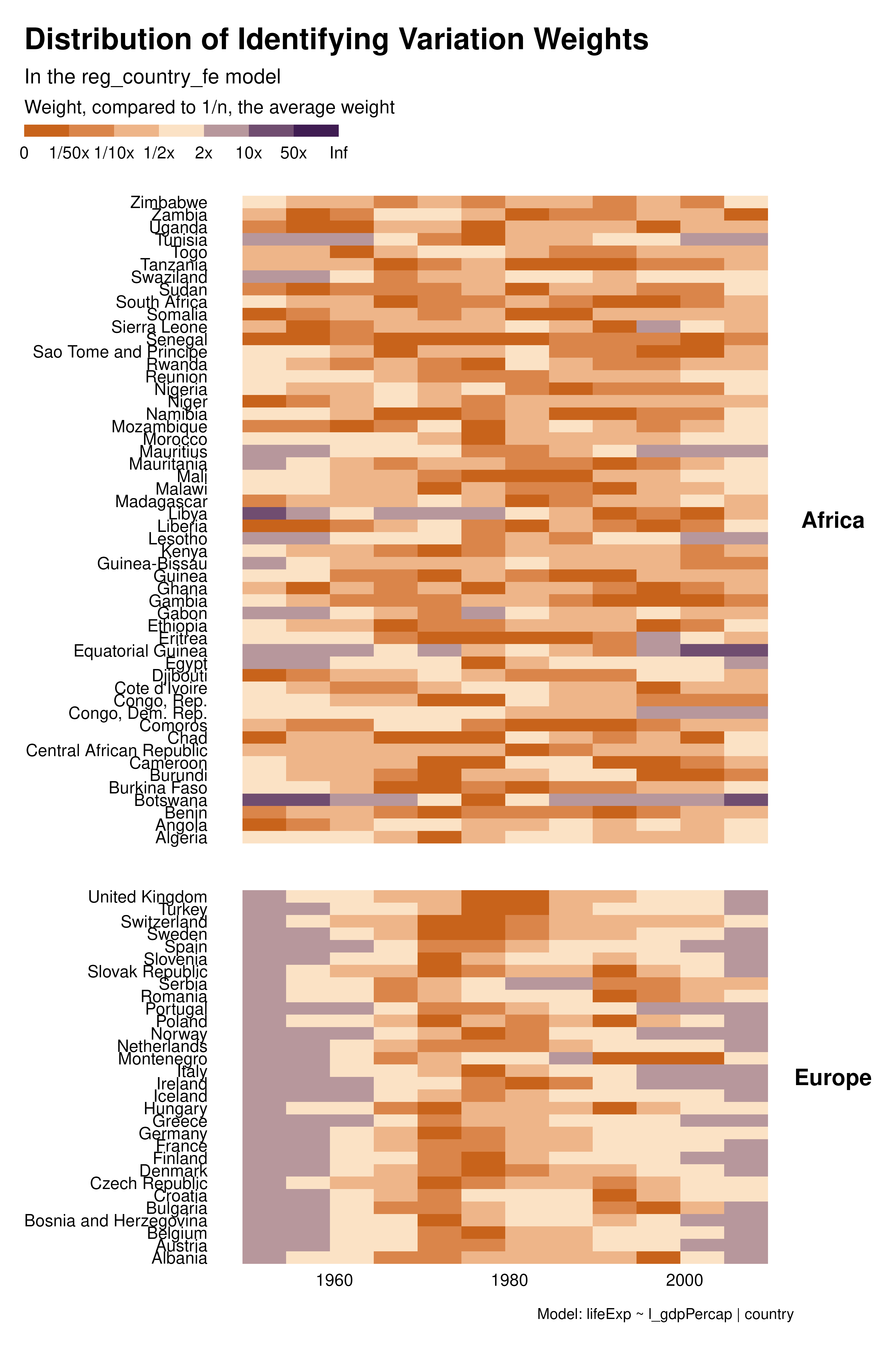
purrr::map(regs, graph_bivar)

Weight graphs

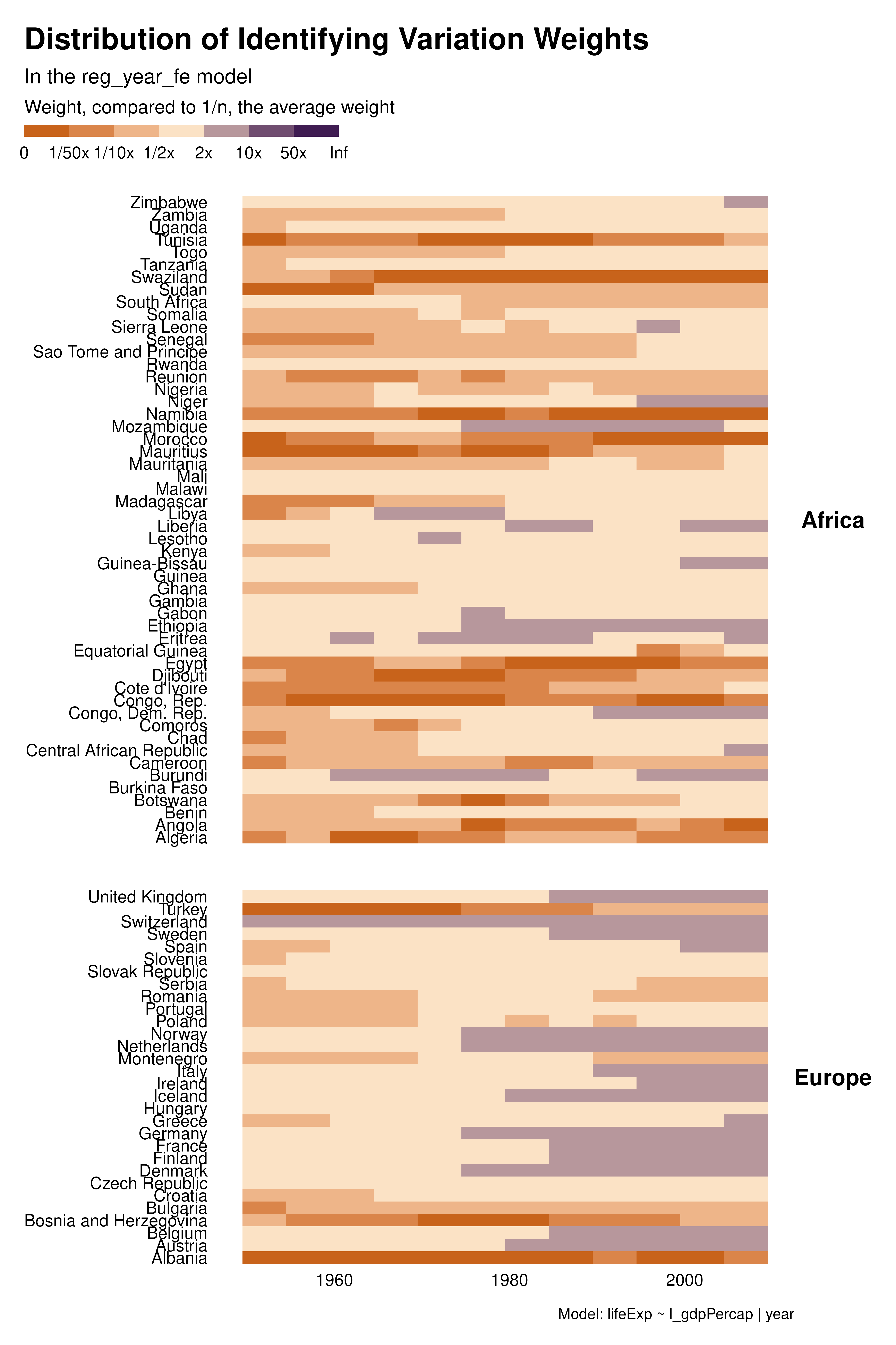
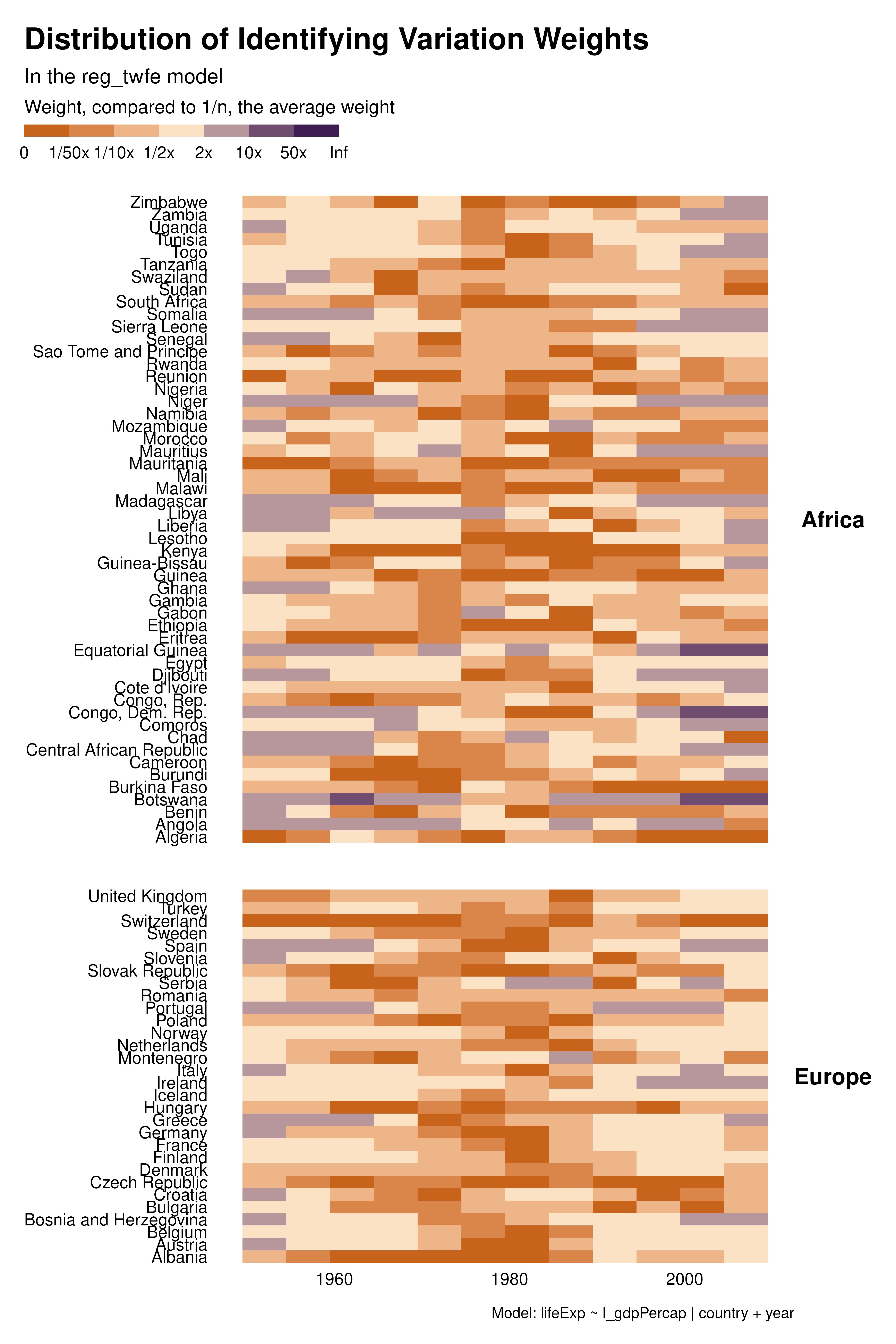
We then explore how different sets of controls/FEs affect the distribution of the weights. The heatmap visualization allows to analyze the contribution of each observation separately and to understand how the individuals weights vary across specifications.

With country or two-ways FEs for instance, many observations, in the for the middle of the period have low weight and therefore contribute little to identification. This is much less the case with year FEs, although later years contribute more. The choice of fixed effects not only affect the estimand but also the weight of observations and therefore the set of observations contributing to identification. In some cases, variation in weights across specifications may be large for some cluster of observations. For instance, a particular specification may focus all the weights on a given set of observations and/or create clusters of low-weight observations.

• Raw
• Continent FEs
• Country FEs
• Year FEs
• TWFE
• Code

graph_weights <- function(reg) {
  reg |> 
    idid_viz_weights("l_gdpPercap", var_x = year, var_y = country) +
    facet_grid(continent ~ ., scales = "free_y", space = "free_y") +
    theme(strip.text.y = element_text(angle = 0)) +
    labs(
      subtitle = paste("In the", deparse(substitute(reg)), "model"),
      caption = paste("Model:", deparse(reg$call[[2]])),
      x = NULL, 
      y = NULL
    )
}

purrr::map(regs, graph_weights)

Contribution graphs

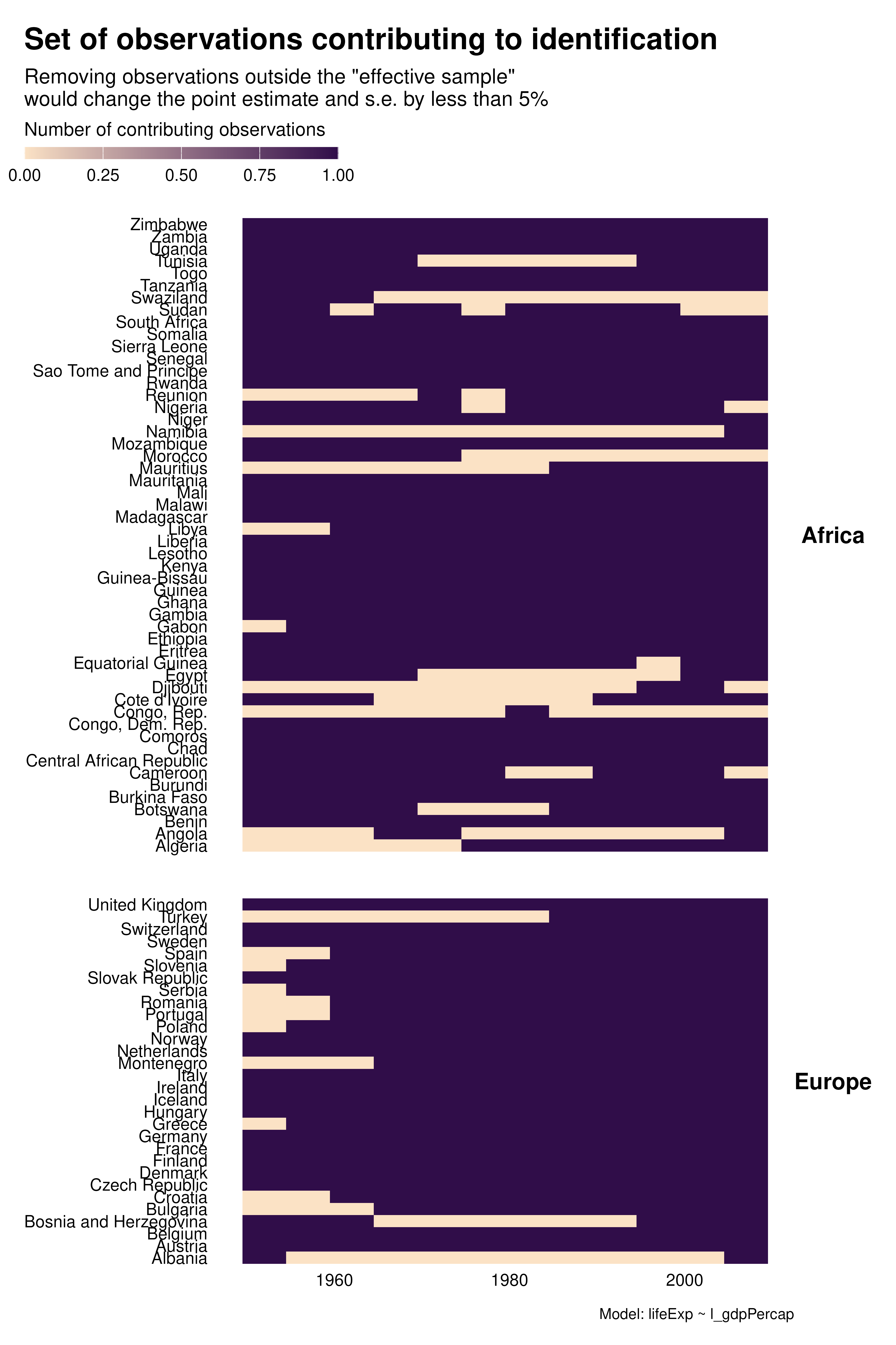
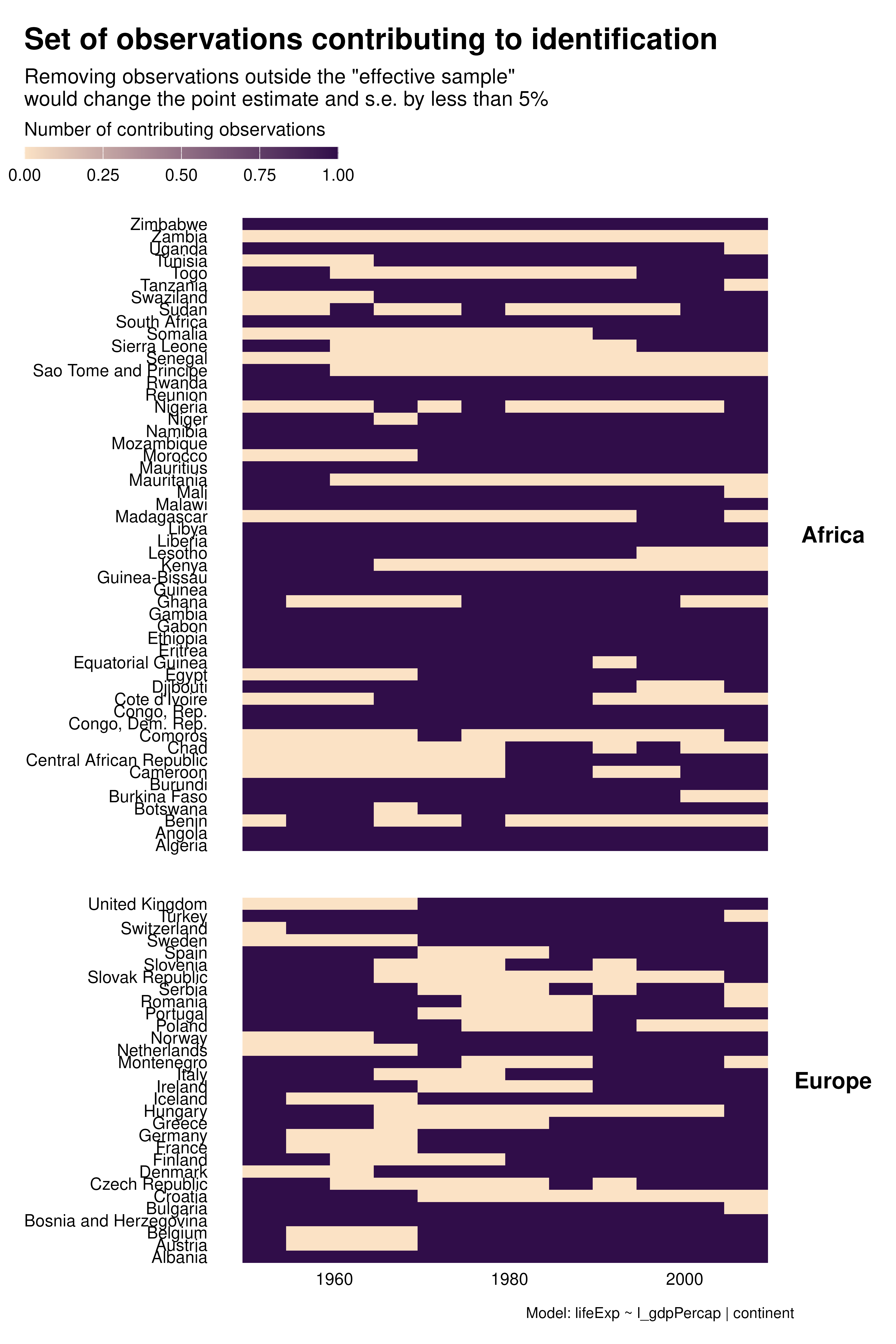
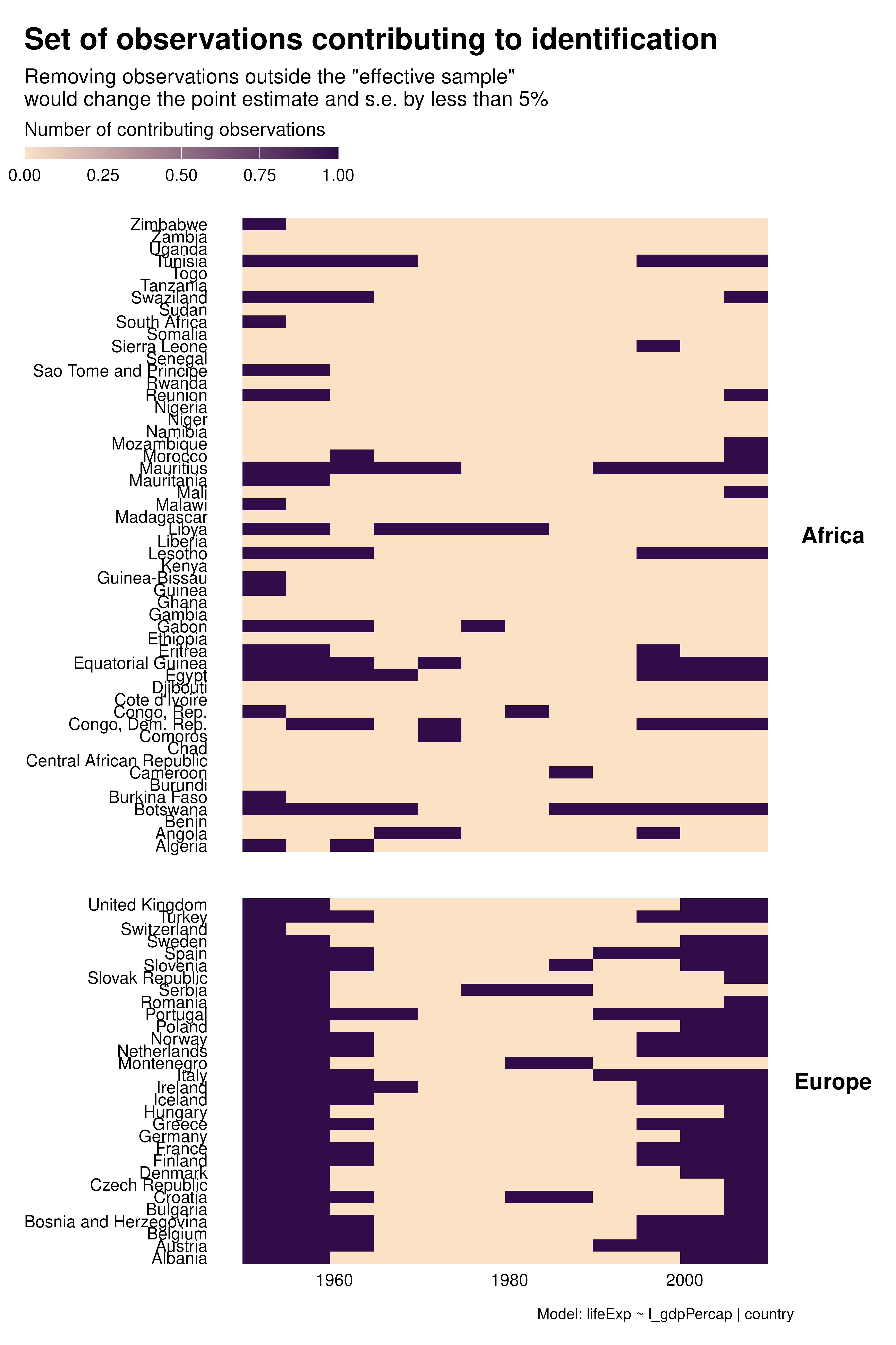
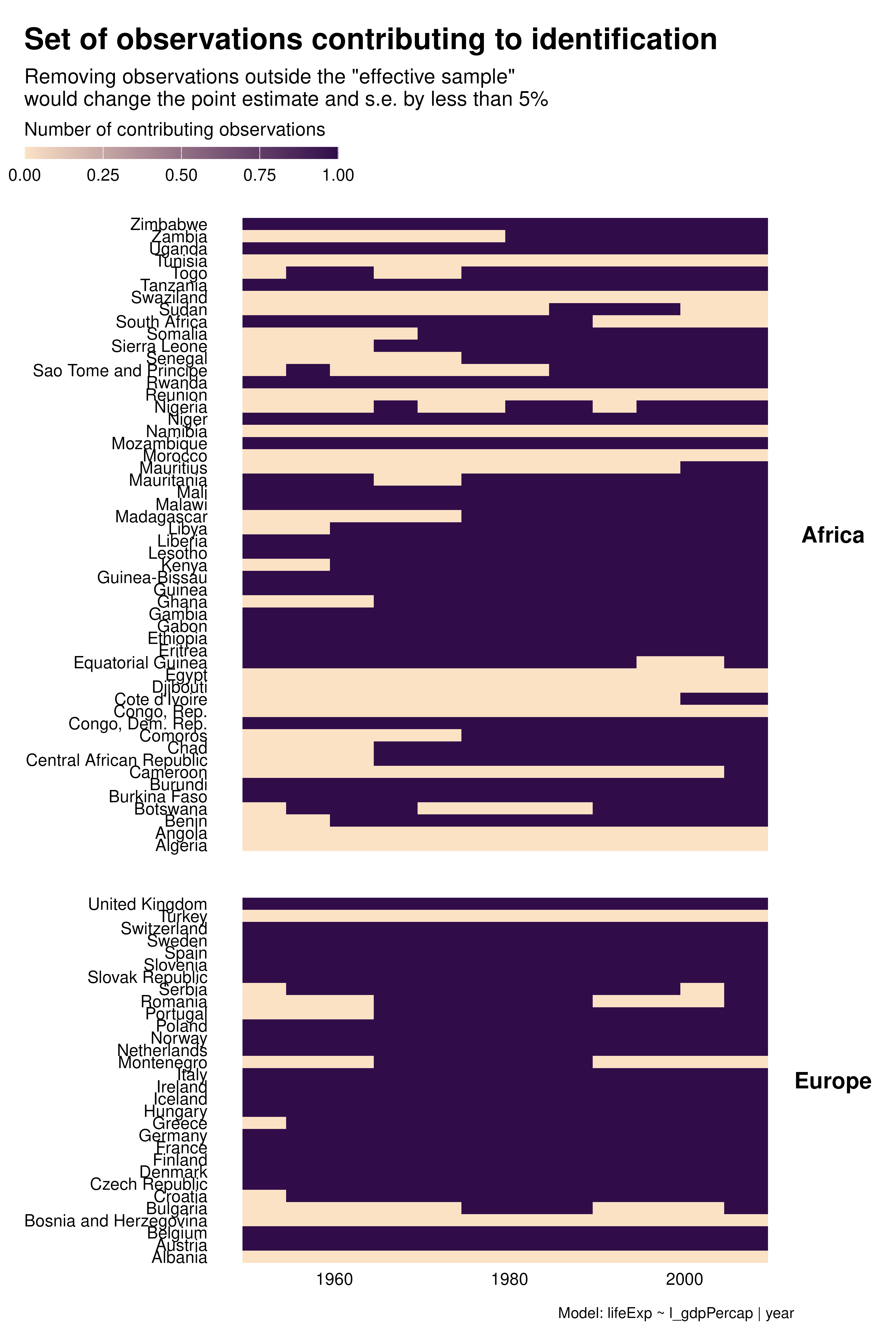
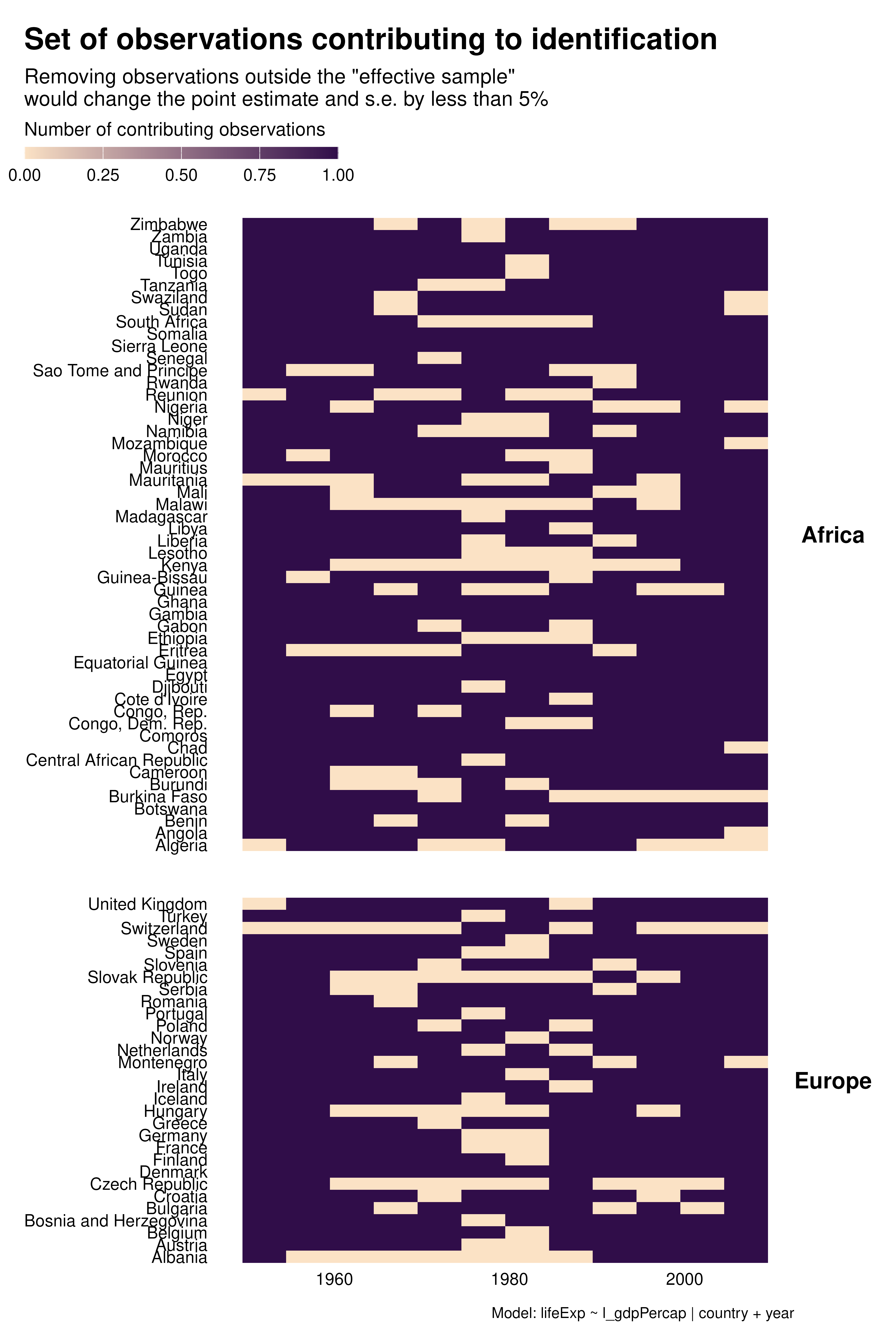
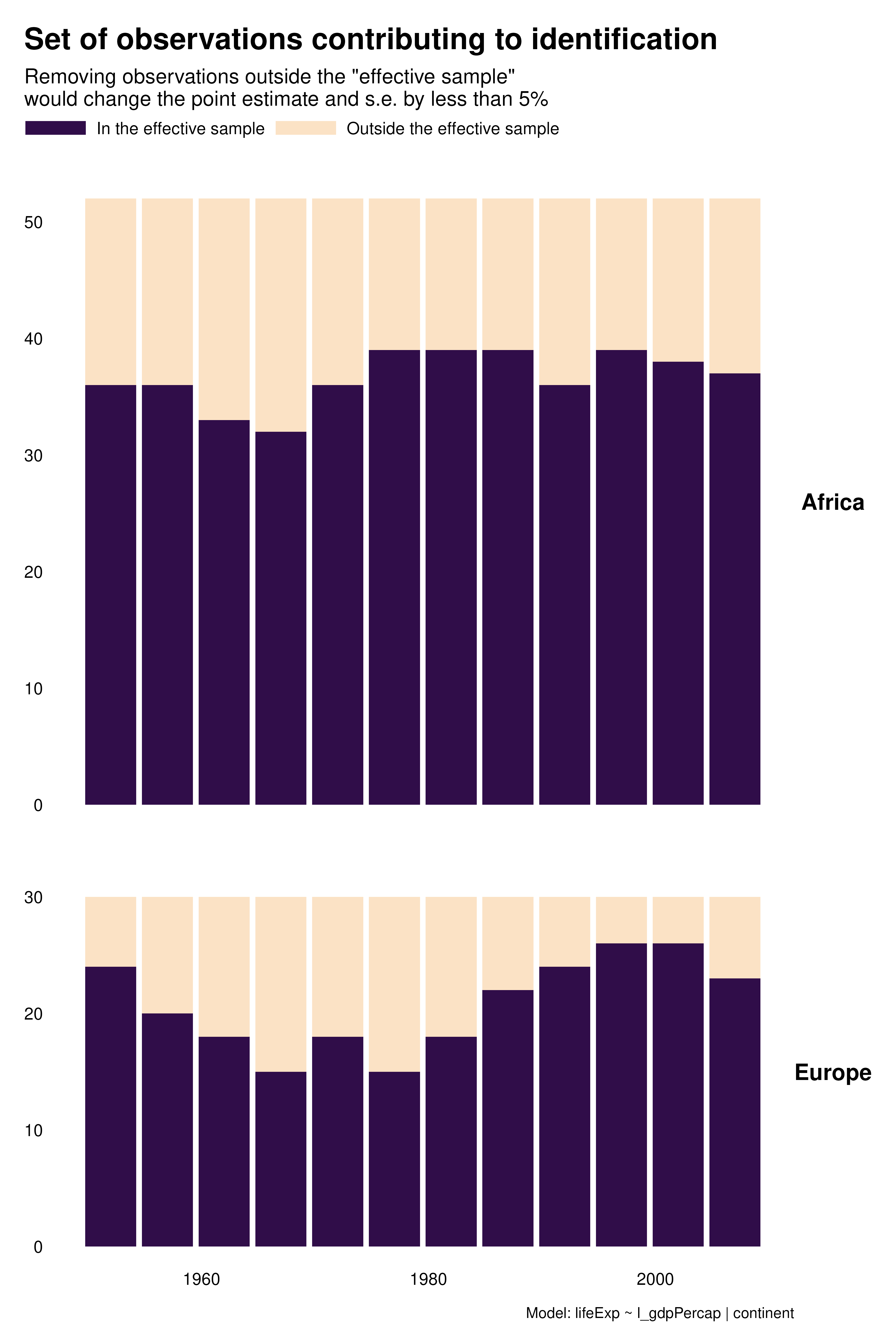
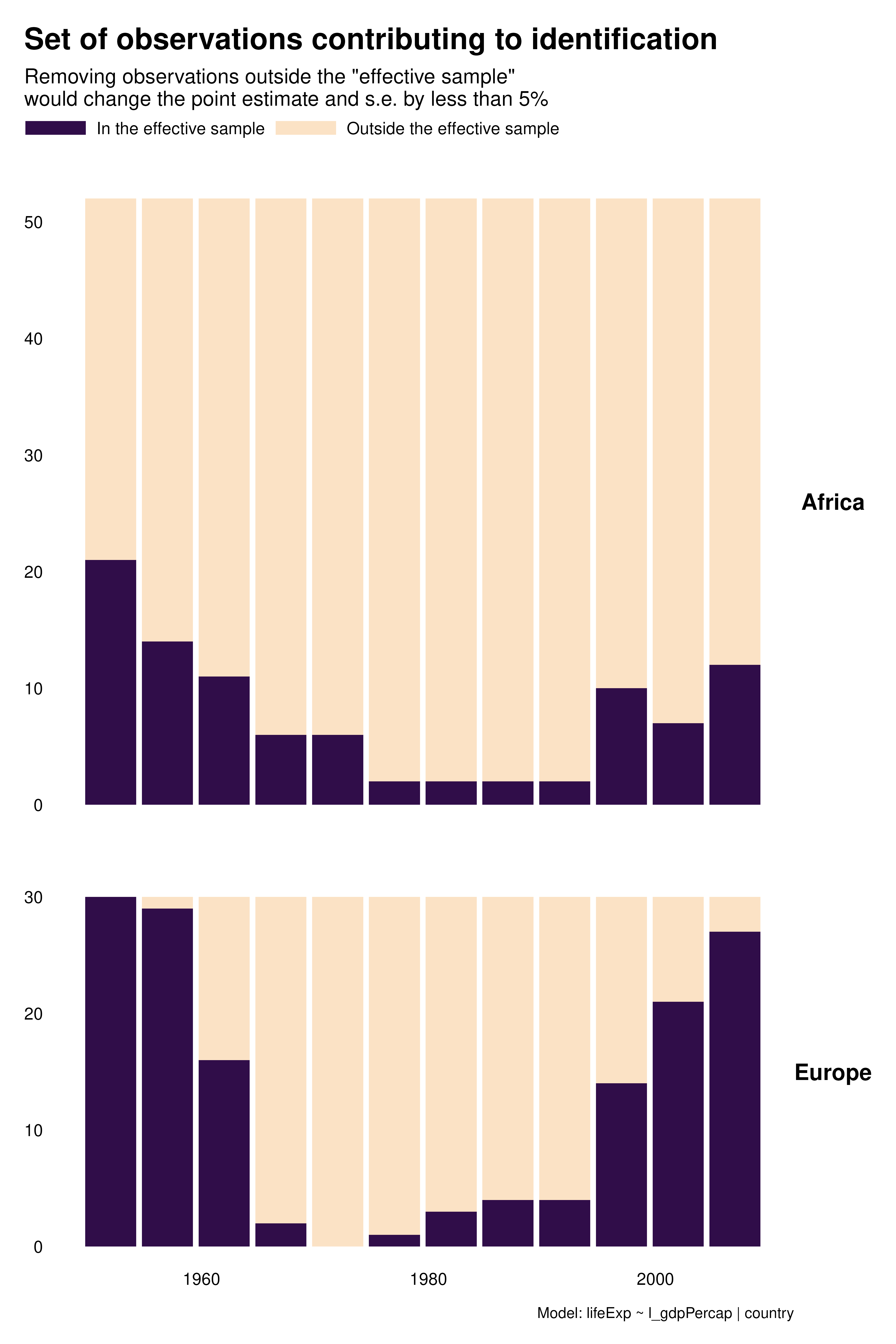
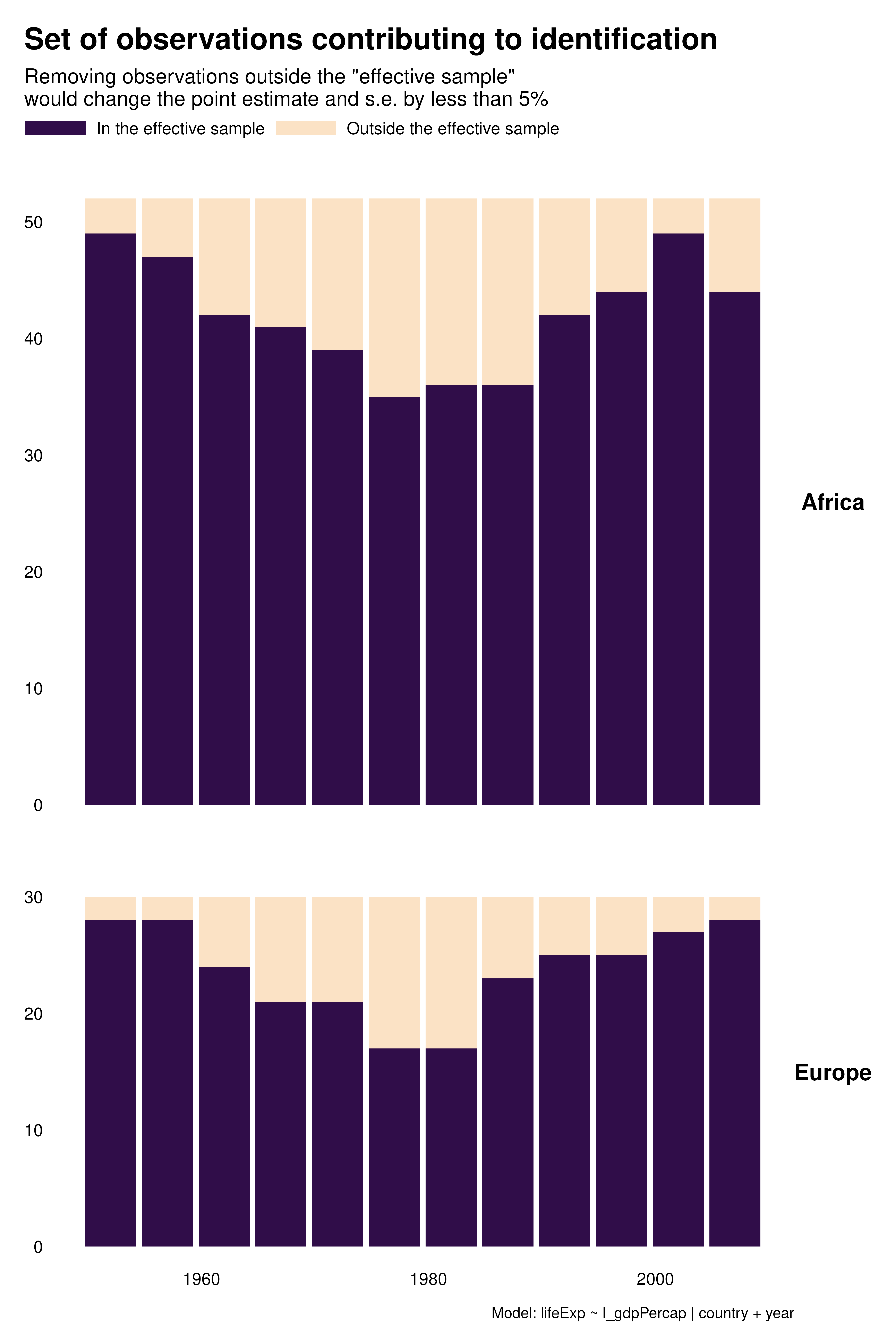
Contribution graphs confirm the previous analyses. They represent observations that one could drop without changing the point estimate and standard error by more than a given proportion, se 5%. With country FEs for instance, not only many observations do not contribute to estimation but observations that do contribute are disproportionately located at the beginning and end of the period. This might affects the external validity of the analysis.

Beyond these external validity concerns, contribution graphs underline that the effective sample size varies a lot across specifications. As discussed in the research paper, specification choices may affect statistical power and exaggeration.

• Raw
• Continent FEs
• Country FEs
• Year FEs
• TWFE
• Code

#> Searching for the contribution threshold

#> Searching for the contribution threshold

#> Searching for the contribution threshold

#> Searching for the contribution threshold

graph_contrib <- function(reg) {
  reg |> 
    idid_viz_contrib("l_gdpPercap", var_x = year, var_y = country) +
    facet_grid(continent ~ ., scales = "free_y", space = "free_y") +
    theme(strip.text.y = element_text(angle = 0)) +
    labs(
      caption = paste("Model:", deparse(reg$call[[2]])),
      x = NULL, 
      y = NULL
    )
}

purrr::map(regs, graph_contrib)

Contribution sets

The previous visual analysis is confirmed by computing the effective sample size; it varies strongly with the specification.

purrr::map(regs, idid_contrib_stats, var_interest = "l_gdpPercap") |> 
  list_rbind() |> 
  mutate(reg = names(regs), .before = 1) |> 
  arrange(n_effective) |> 
  knitr::kable()

reg	n_initial	n_nominal	n_effective	prop_effective
reg_country_fe	984	984	246	0.2500000
reg_continent_year_fe	984	984	542	0.5508130
reg_continent_fe	984	984	689	0.7002033
reg_year_fe	984	984	689	0.7002033
reg_twfe	984	984	788	0.8008130
reg_raw	984	984	837	0.8506098

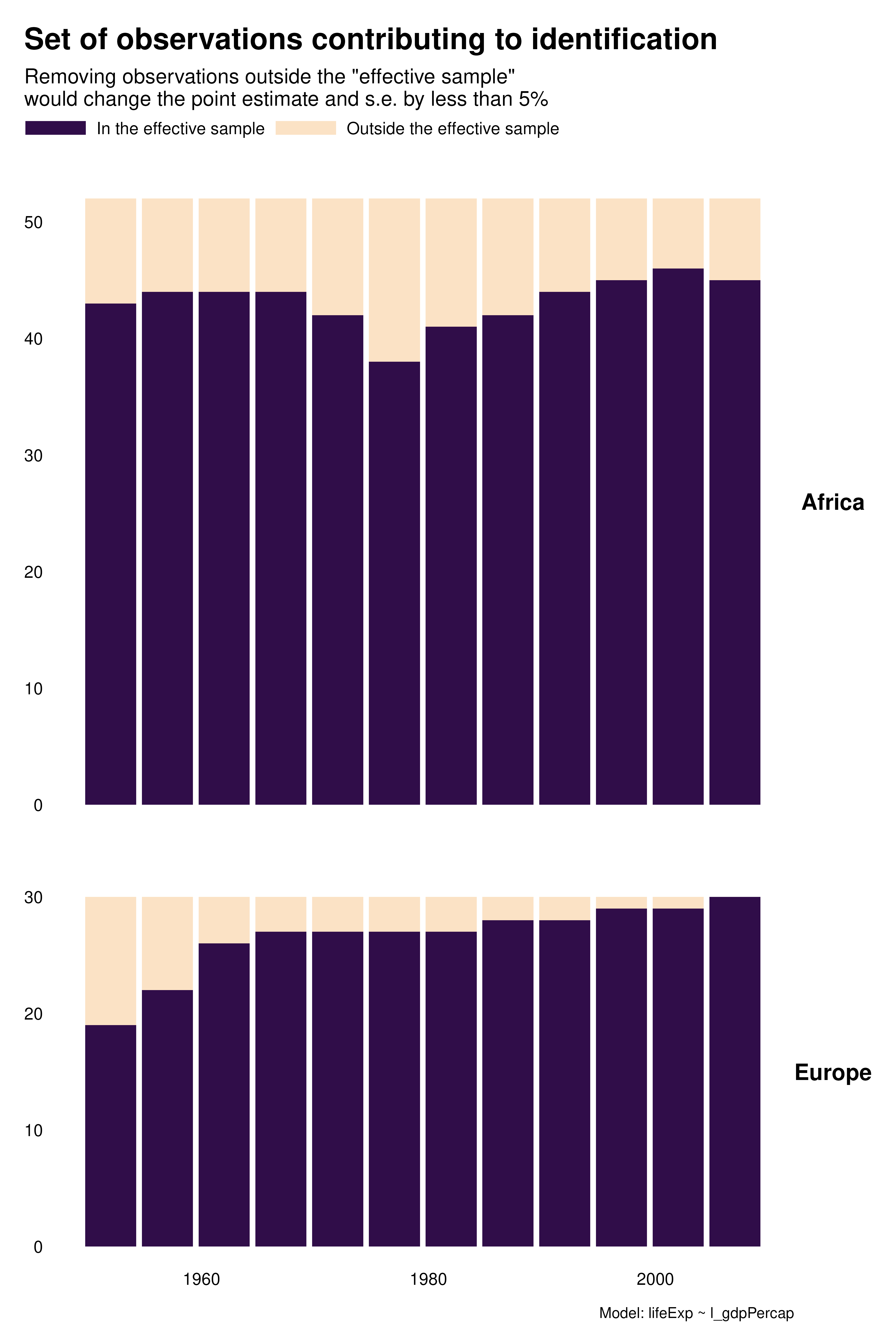
Histograms

A substantial share of the variation across specifications seem to come from time. We can explore this further by focusing on this variable and building histograms instead of heatmaps. As noted above, for country FEs, most of the contributing observations are located in early and late periods. In addition, there is a notable pattern with year FEs for Africa: later years contribute more than earlier years.

• Raw
• Continent FEs
• Country FEs
• Year FEs
• TWFE
• Code

#> Searching for the contribution threshold

#> Searching for the contribution threshold

#> Searching for the contribution threshold

#> Searching for the contribution threshold

hist_contrib <- function(reg) {
  reg |> 
    idid_viz_contrib("l_gdpPercap", var_x = year) +
    facet_grid(continent ~ ., scales = "free_y", space = "free_y") +
    theme(strip.text.y = element_text(angle = 0)) +
    labs(
      caption = paste("Model:", deparse(reg$call[[2]])),
      x = NULL, 
      y = NULL
    )
}

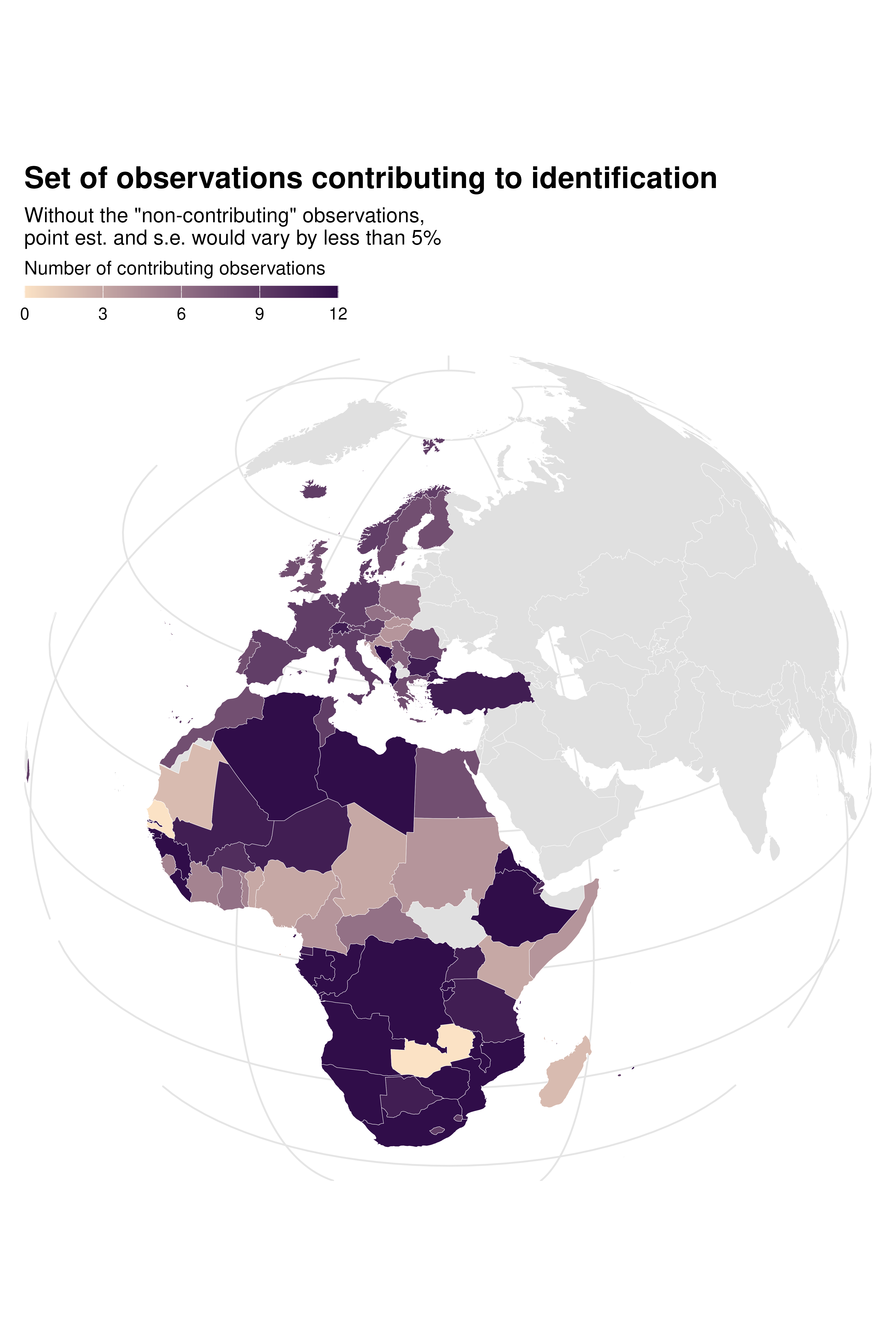
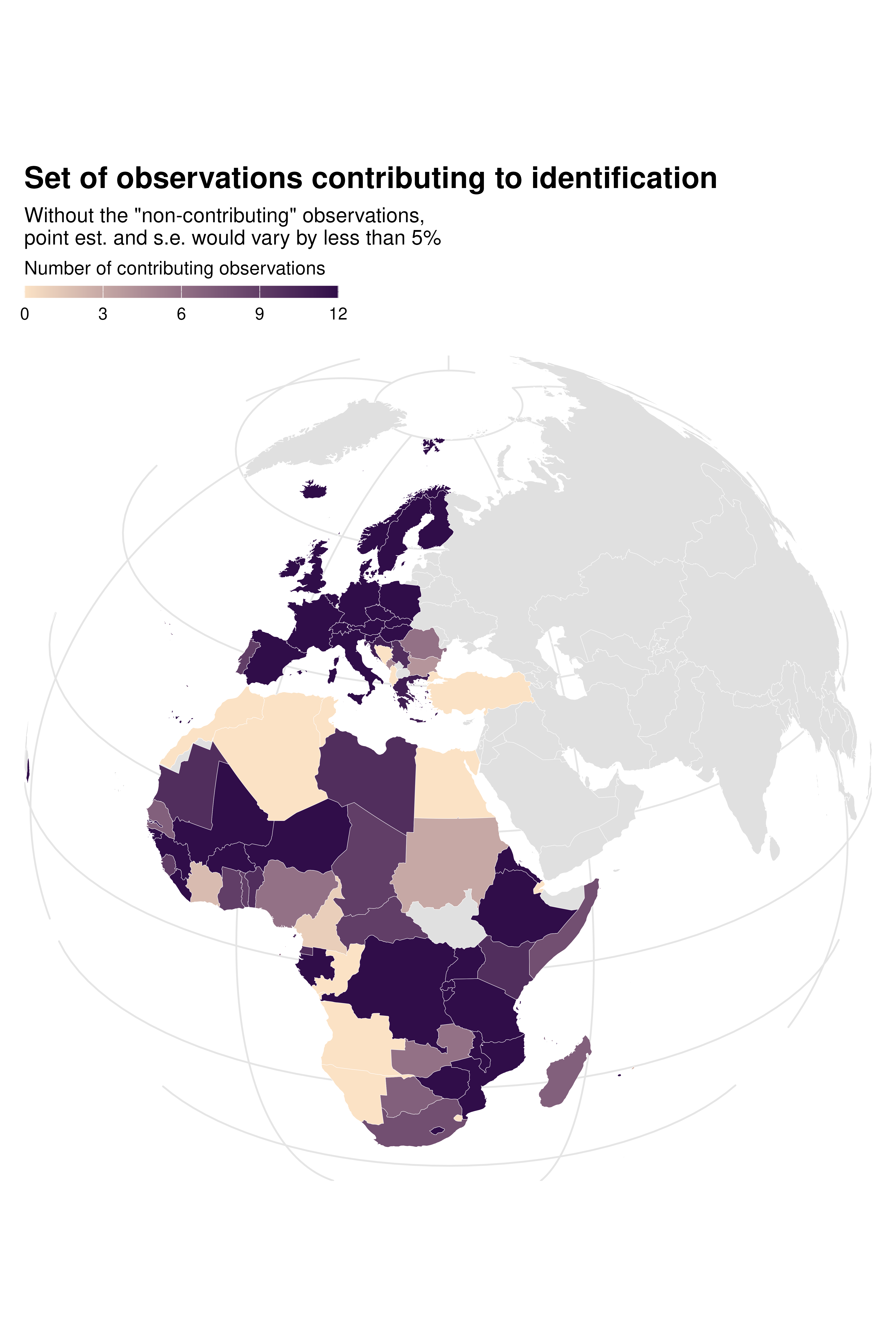
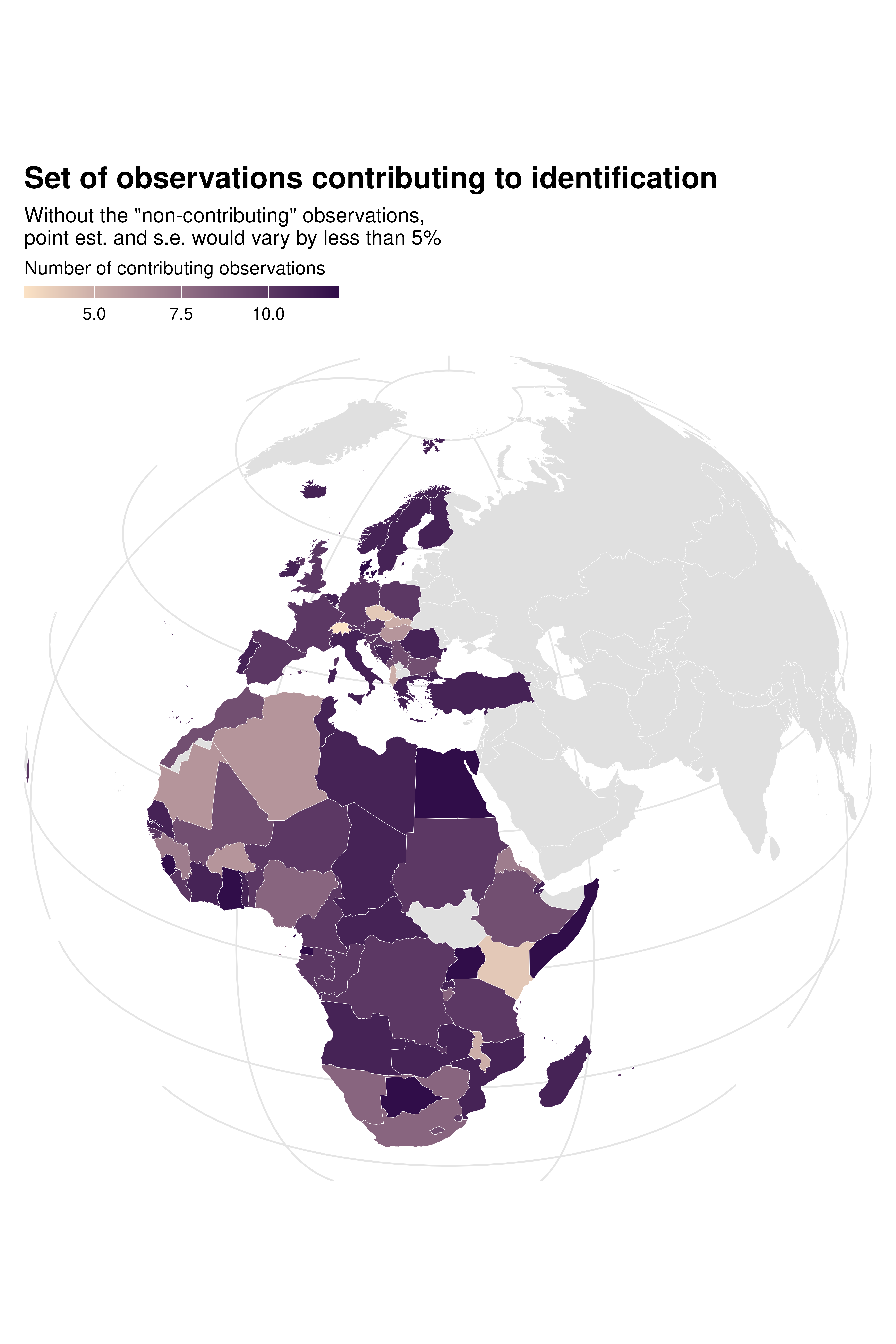
purrr::map(regs, hist_contrib)

Maps

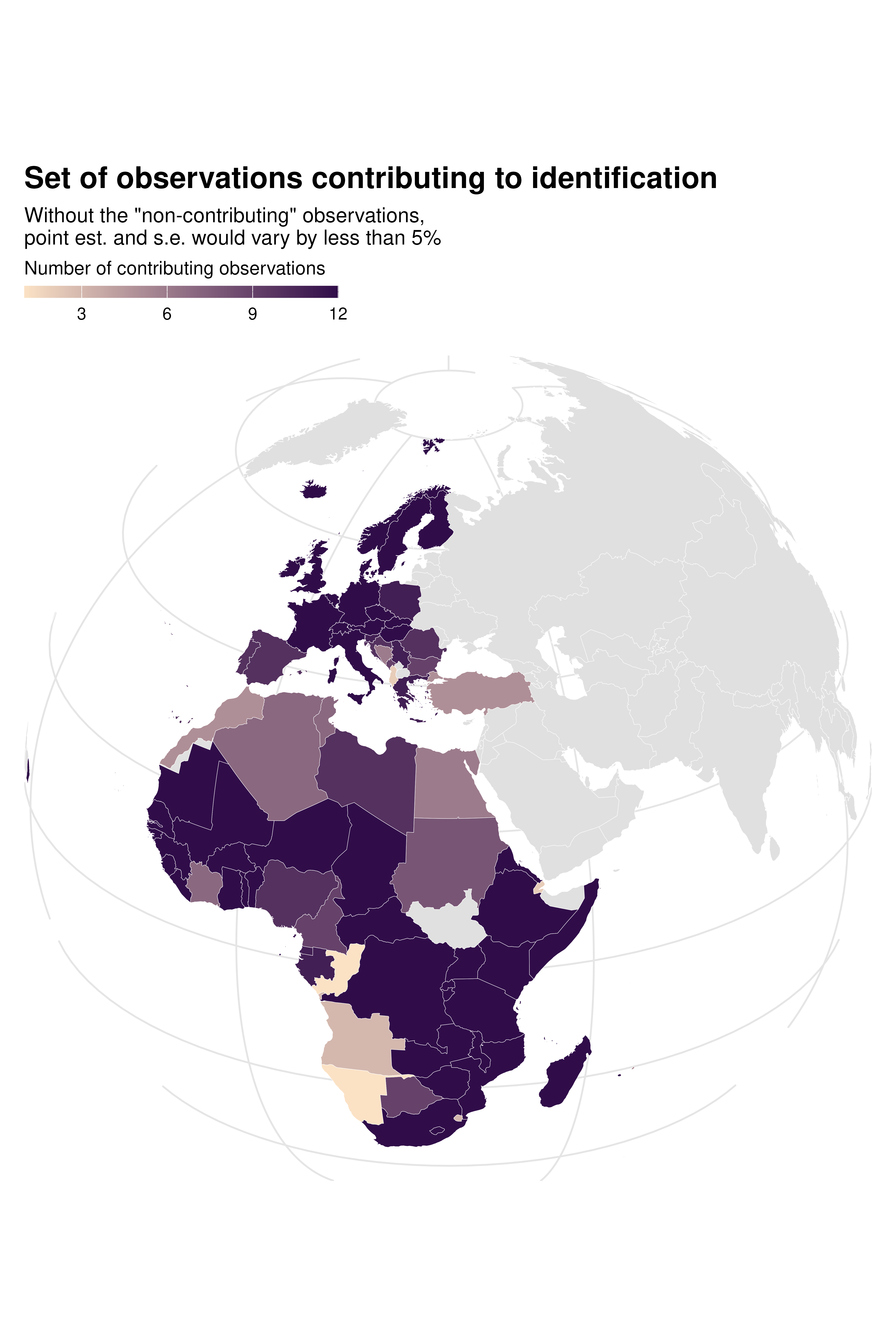
Since there is also variation across specifications in terms of how much each country contributes to identification, we can use idid_viz_map to explore this further. In the country FE specification, the set of countries that contribute to identification is limited and not representative of the overall sample.

• Raw
• Continent FEs
• Country FEs
• Year FEs
• TWFE
• Code

#> Searching for the contribution threshold

#> Searching for the contribution threshold

#> Searching for the contribution threshold

#> Searching for the contribution threshold

world_sf <- rnaturalearth::ne_countries(scale = "medium", returnclass = "sf") |> 
  mutate(iso_alpha = adm0_a3)

map_contrib <- function(reg) {
  idid_viz_contrib_map(reg, "l_gdpPercap", world_sf, "iso_alpha") +
    coord_sf(crs = "+proj=ortho +lon_0=30 +lat_0=28", expand = FALSE) +
    theme(panel.grid.major = element_line(colour = "gray90")) 
}

purrr::map(regs, map_contrib)

Conclusion

Overall, this analysis showed issues of representativity and effective sample size in the country FEs specification. It invites to consider the results from this specification carefully.