What is exaggeration?
Exaggeration is one of the key concepts in the present paper. To understand how low statistical power can cause exaggeration in the presence of publication bias, let’s analyze replications of laboratory experiments in economics ran by Camerer et al (2016).
First, I retrieve their replication results, alongside the results of the initial studies, from their project website. I just ran their Stata script create_studydetails.do to generate their data set. Since the standard errors of the estimates are not reported in this data set, I recompute them.
First, I focus on one particular study, Abeler et al. (2011), in order to illustrate in more details the issue of interest. I first plot in red the estimate and 95% confidence interva Abeler et al. obtained in their experiment (note that I will run replications and there will be several draws of estimates in subsequent graphs, hence why the x-axis of the graph below):
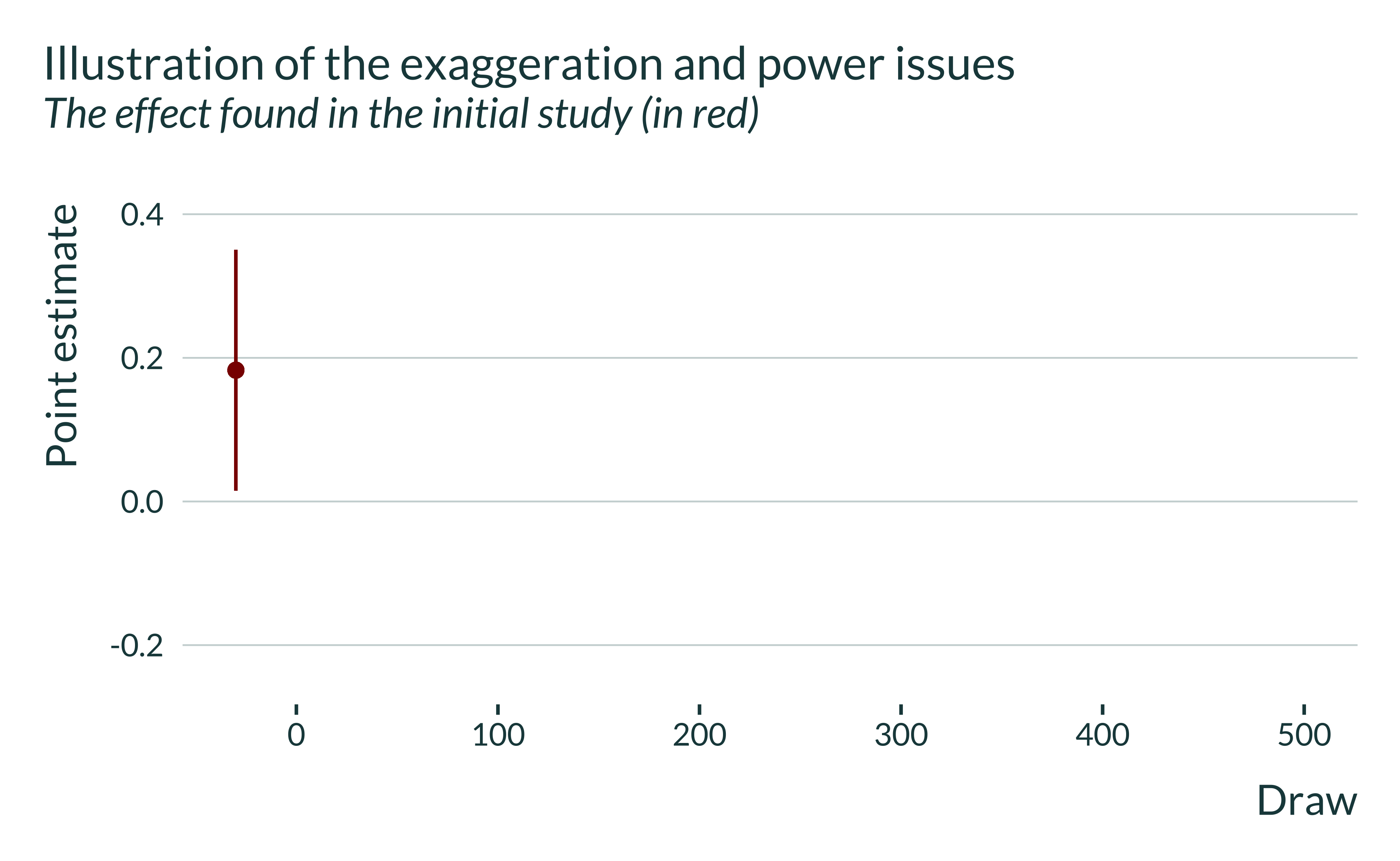
This estimate is significant and has been published. Yet, it is pretty noisy.
I then plot the result of the replication in blue:
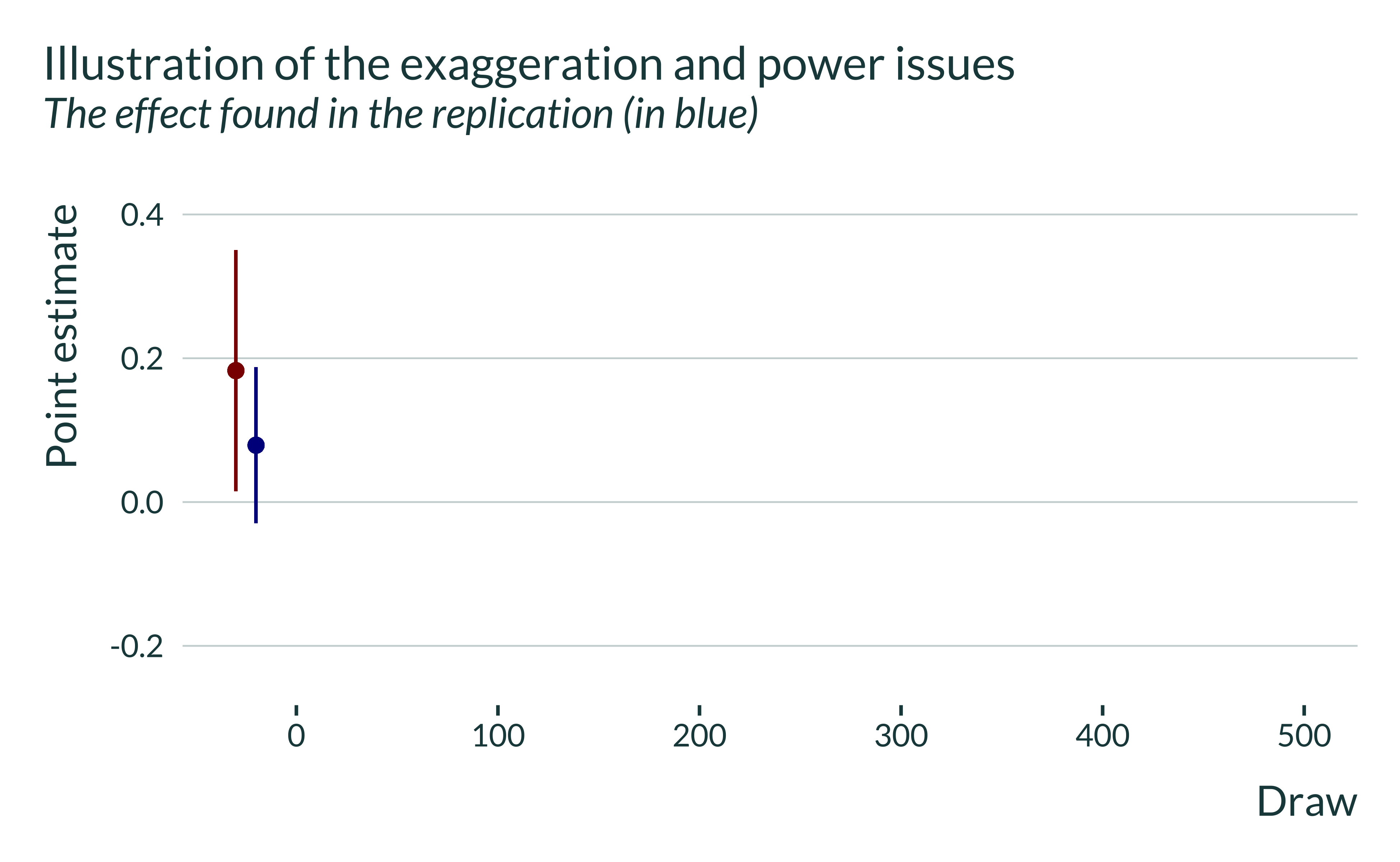
This estimate is both more precise and smaller than the initial one. It still remains noisy and it is not statistically significant.
Let’s now assume that the true effect is actually equal to this replicated estimate. Would the design of the initial study be good enough to detect this effect? ie if we replicated the initial study, could we reject the null of no effect, knowing that the true effect is equal to the replicated estimate?
To illustrate this, I first plot in gray the point estimate form the replicated study but with a standard error equal to the initial study’s, i.e. approximately the estimate that would have been obtained with the design of the initial study but with an effect equal to the replicated one. This emulates what would have yielded a replication of the initial study if the true effect was equal to the replication estimate.
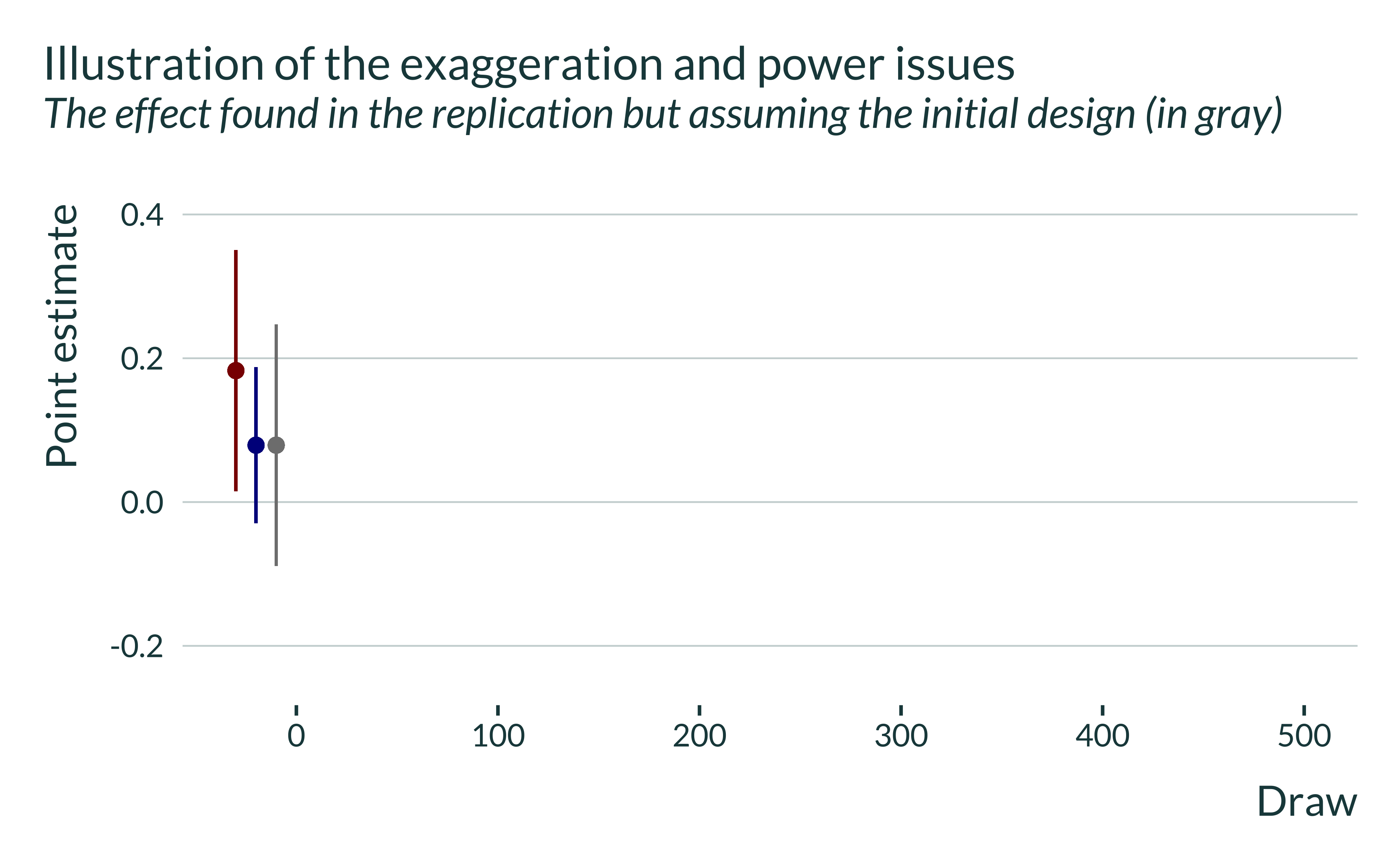
This estimate is non significant. In this instance, we would not have been able to reject the null of no effect. Now, let’s replicate this study 500 times, running 500 lab experiments with the design of the initial study and under the assumption of a true effect equal to the one obtained in the replication:
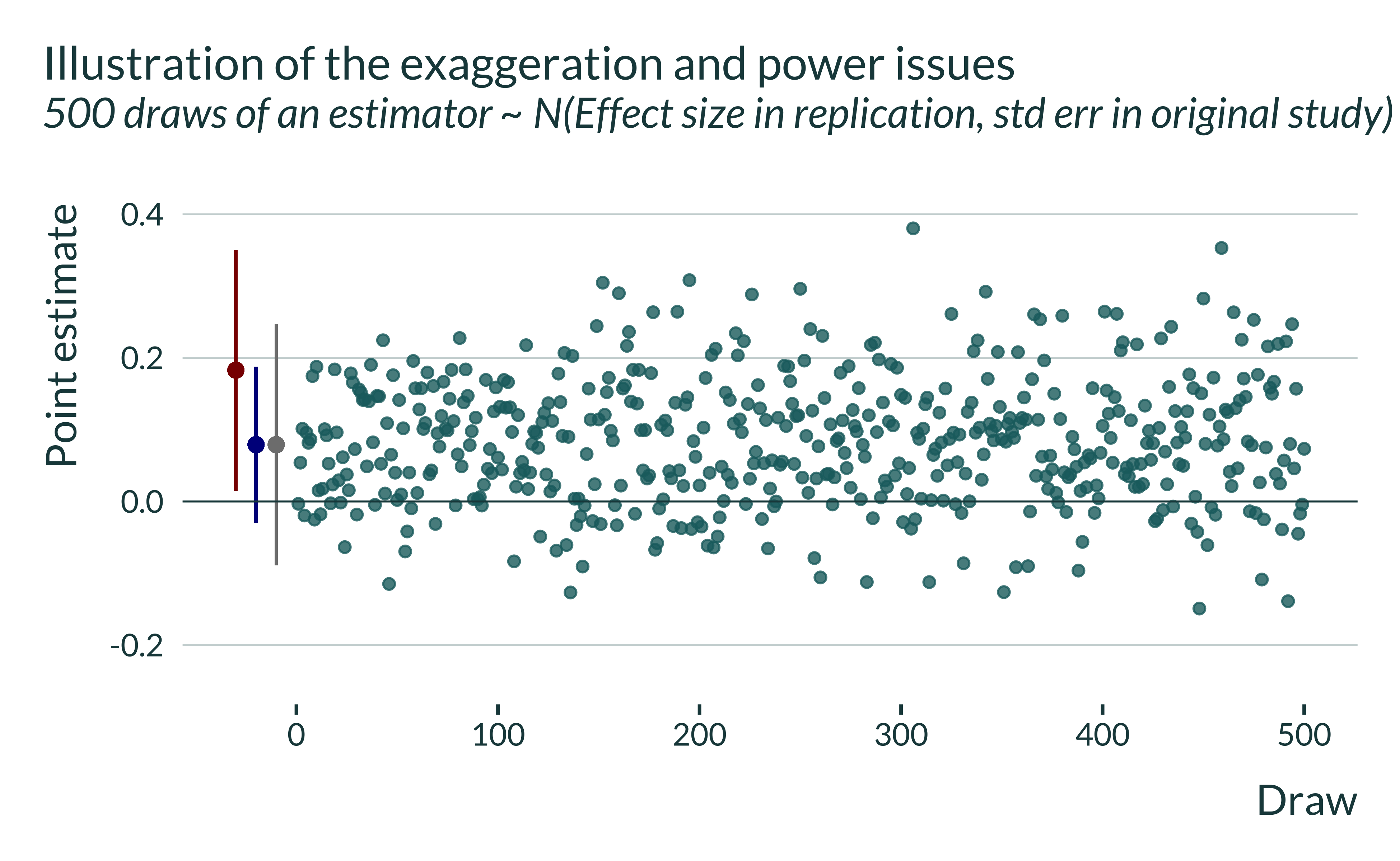
The distribution is centered on the “true effect” (i.e., the point estimate found in the replication study) and has a standard deviation equal to the standard error of the estimator of the original study. Let’s now condition on statistically significance:
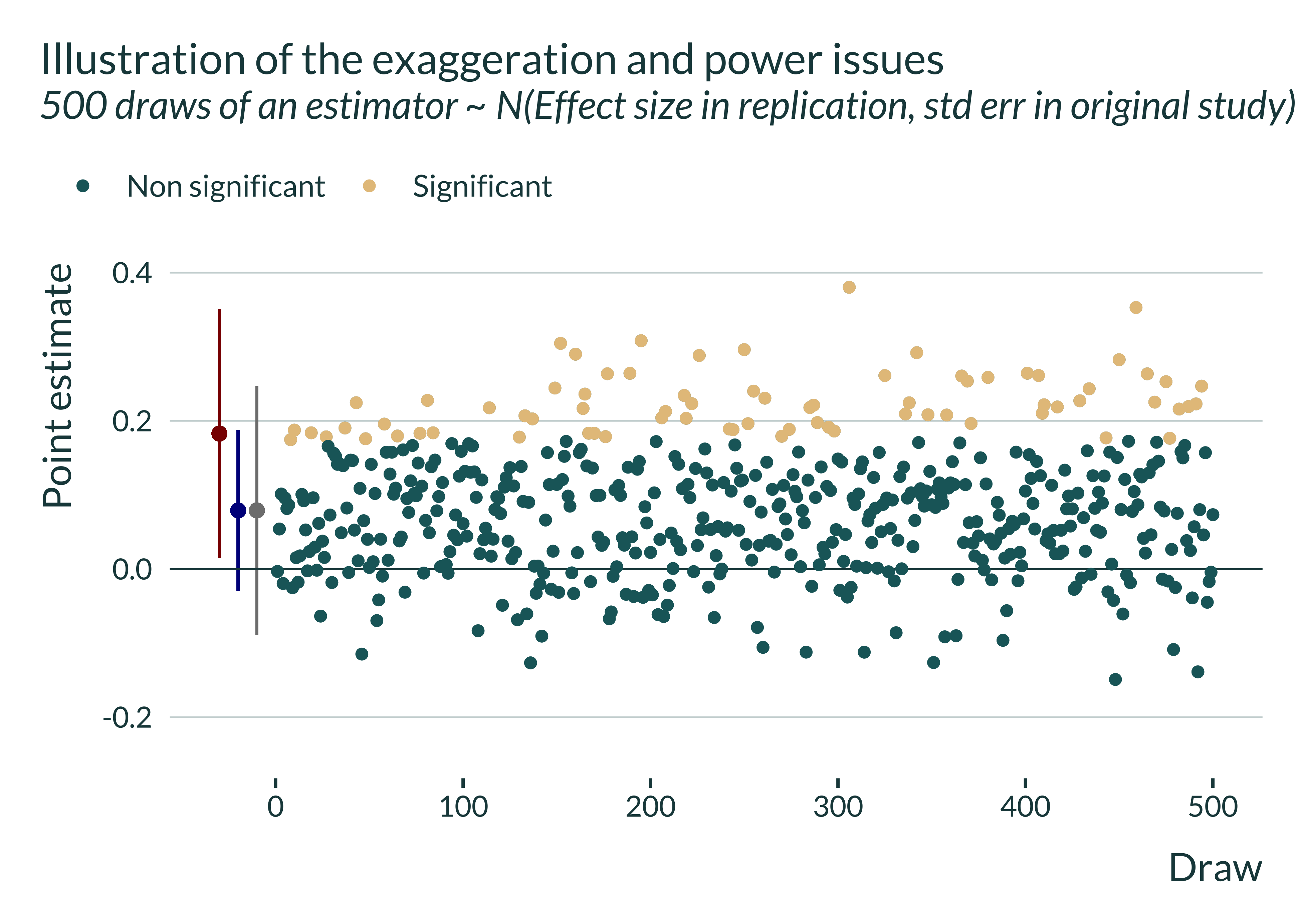
In some cases we would get statistically significant estimates (the beige dots) and non statistically significant ones (the green dots) in others cases. The statistical power here is basically the proportion of statistically significant estimates.
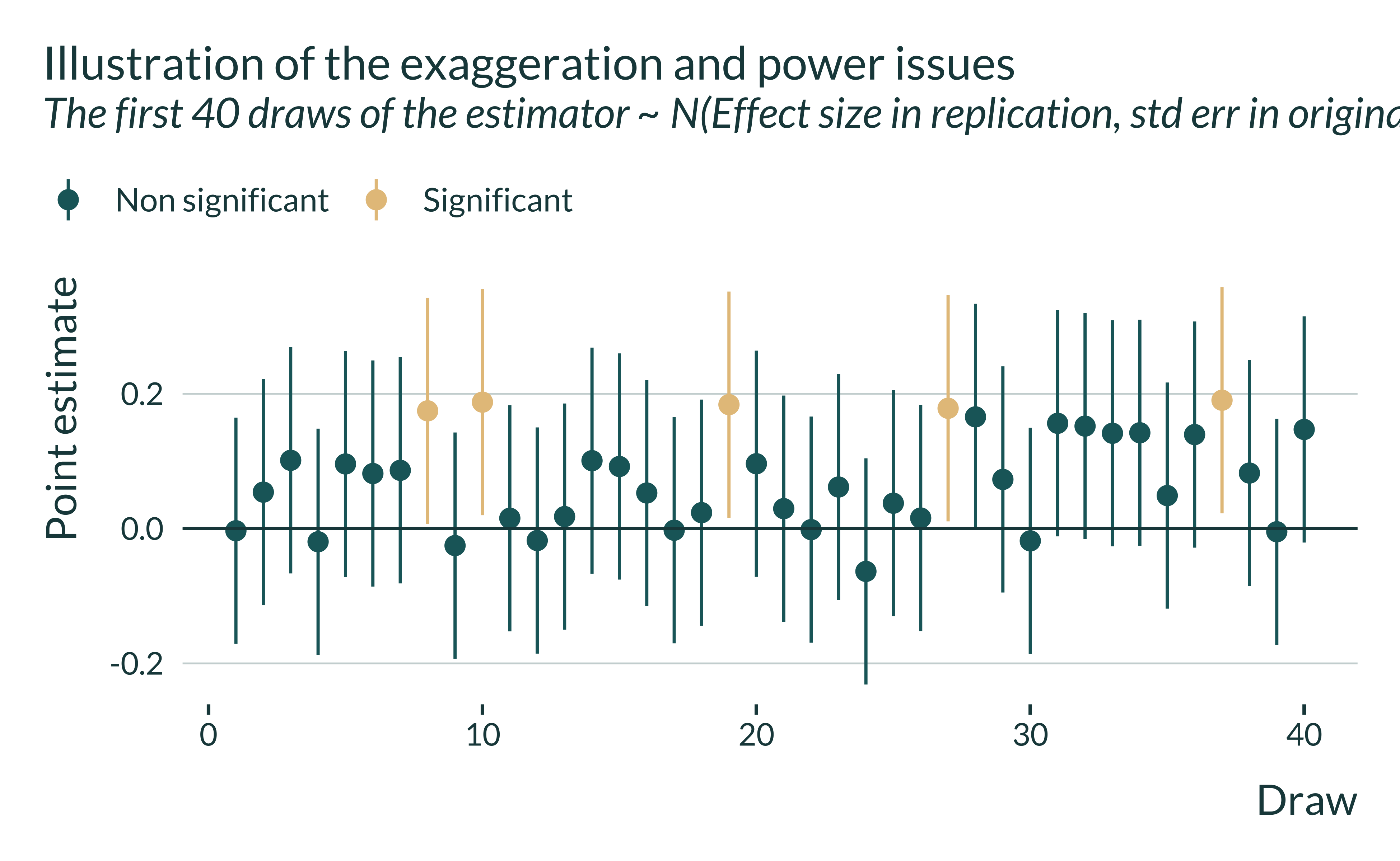
Zooming in on the first draws and plotting their 95% confidence intervals (approximately \([\hat{\beta} - 1.96 \cdot \sigma_{\hat{\beta}}, \hat{\beta} + 1.96 \cdot \sigma_{\hat{\beta}}]\)) helps understand why some estimates are deemed significant and not others. By definition, significant estimates are those whose confidence interval does not contain 0:
If the study was more precise, the standard error of the estimator would be smaller and more estimates would be statistically significant. The study would have more statistical power. But since the power is low here (or equivalently since the estimator is relatively imprecise), statistically significant estimates only represent a subset of the estimate and on average overestimate the true effect. They overestimate it by a factor 2.847443 (average of 0.2251483 while the true effect is 0.0790704).
On average, statistically significant estimates overestimate true effect sizes when statistical power is low.
Why does imprecision lead to exaggeration?
The confounding / exaggeration trade-off described in this paper arises due to differences in precision between estimators. To illustrate this, I generate estimates from two unbiased estimators with identical mean but different variances.
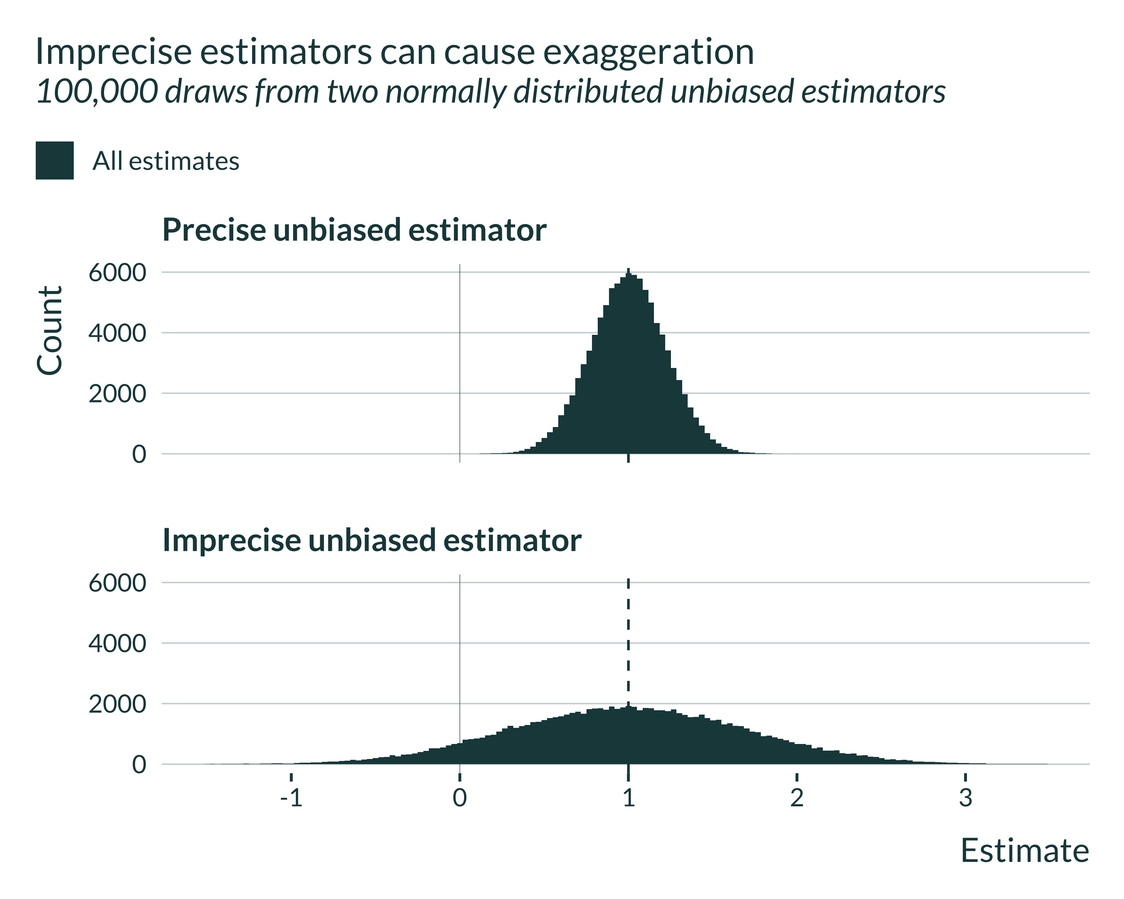
Both estimators, since unbiased, are centered on the true effect, here 1. The distribution of the imprecise estimator is by definition more spread out.
Let’s then have a look at which estimates are statistical significant and which are not. To be significant, estimates have to be at least 1.96 standard errors away from 0. Thus, for the imprecise estimator, they have to be further away from 0:
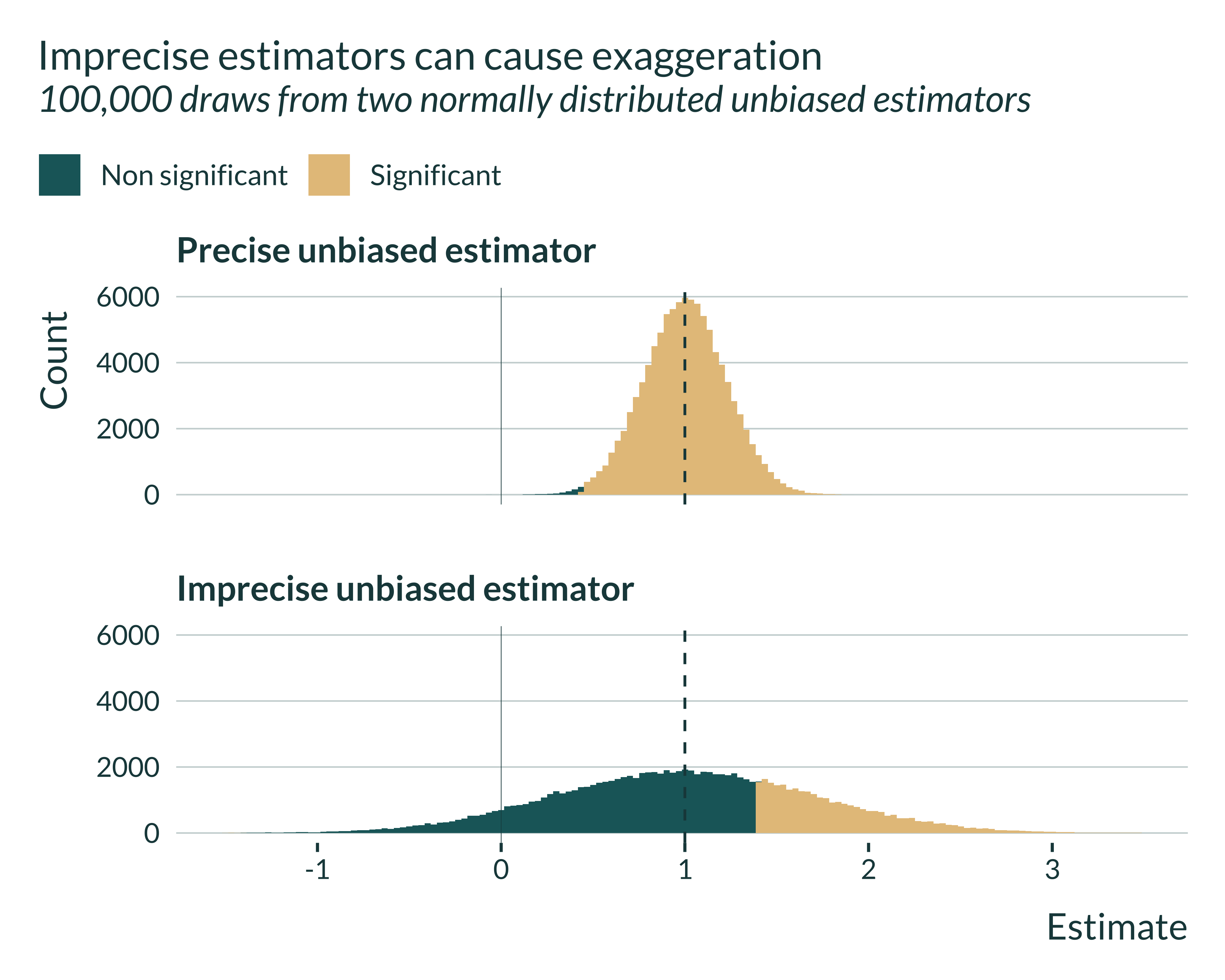
We notice that for the precise estimator, most estimates are statistically significant. The 1.96 standard errors threshold is not very far from 0. This is very different for the imprecise estimator: significant estimates are located in the tails of the distribution.
If we look at the mean of these significant estimates, it is almost equal to the true effect in the case of the precise estimator but quite different for the imprecise estimator:

Even though the estimator is unbiased, the set of statistically significant estimates is a biased sample of the distribution.
Note that this figure also suggests that, the less precise the estimator, the larger the exaggeration.
Do we actually see exaggeration in the literature?
I then describe evidence of exaggeration found by Camerer et al. Out of the 18 studies, 3 replications have opposite signs as compared to the original study. Out of those that are of the same sign, original studies are on average 1.5845684 larger than replicated ones.
The number and proportion of original studies that were statistically significant are as follows:
| Original estimate statistically significant | Number | Proportion |
|---|---|---|
| No | 2 | 0.11 |
| Yes | 16 | 0.89 |
For the replication studies, these statistics are as follows:
| Replication estimate statistically significant | Number | Proportion |
|---|---|---|
| No | 7 | 0.39 |
| Yes | 11 | 0.61 |
Now, I want to compute the statistical power of the initial analysis. To do so, we need to assume a value of the true effect. I assume that this true effect is equal to the effect found in the replication and compute the corresponding statistical power and exaggeration of the original study using the retrodesign package.
The distribution of the exaggeration ratio and power are as follows:
Show the code used to generate the graph
retro_camerer %>%
  ggplot() +
  geom_dotplot(aes(x = type_m), color = NA) +
  labs(
    title = "Distribution of the exaggeration ratio in the original studies",
    subtitle = "If the true effect was equal to the replicated one",
    x = "Exaggeration ratio (log scale)",
    y = "Number of studies",
    caption = "Each dot represents one study"
  ) +
  scale_x_log10() +
scale_y_continuous(NULL, breaks = NULL) 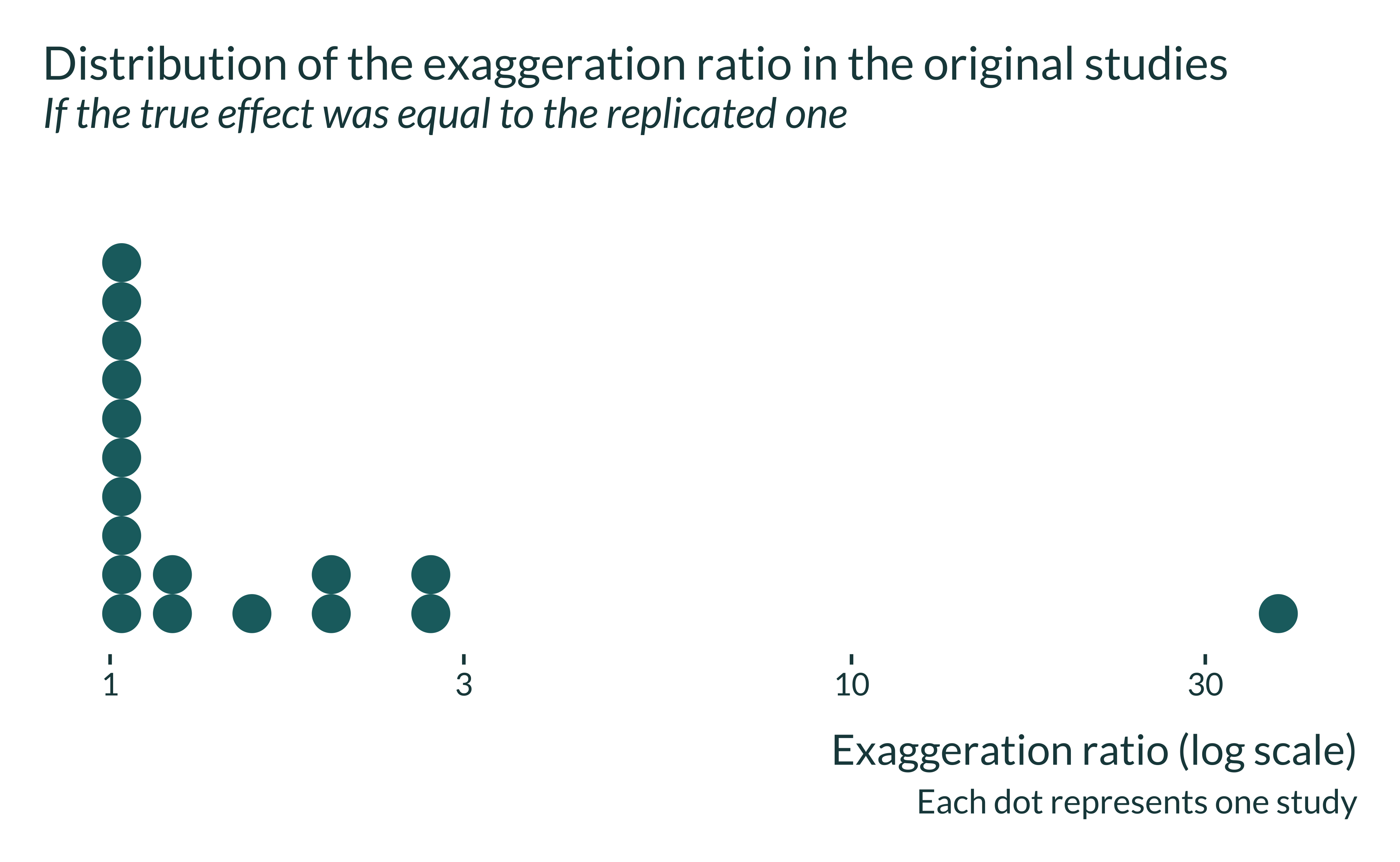
Show the code used to generate the graph
retro_camerer %>%
  ggplot() +
  geom_dotplot(aes(x = power*100), color = NA) +
  labs(
    title = "Distribution of the power in the original studies",
    subtitle = "If the true effect was equal to the replicated one",
    x = "Power (%)",
    y = "Number of studies",
    caption = "Each dot represents one study"
  ) +
scale_y_continuous(NULL, breaks = NULL) 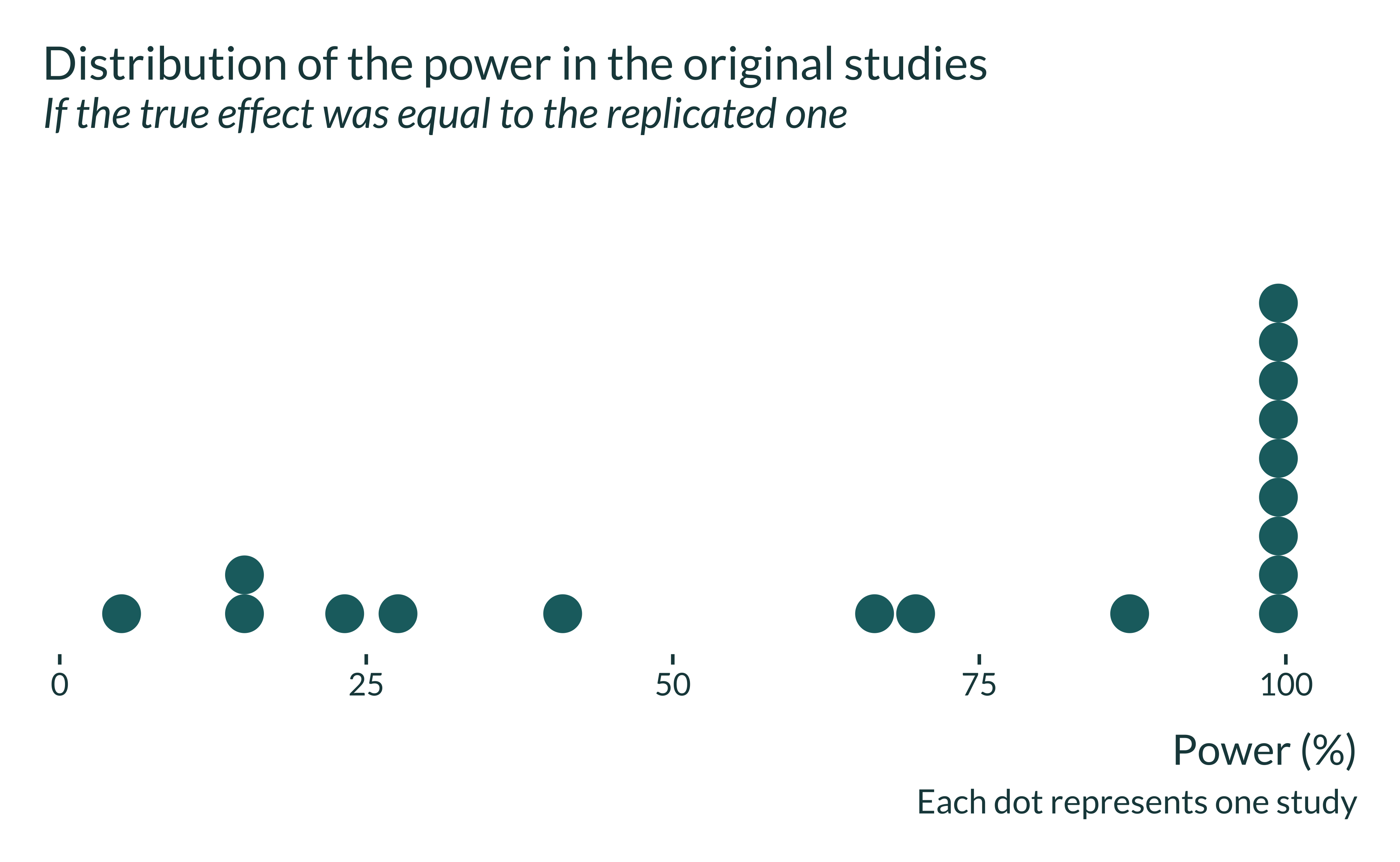
Show the code used to generate the graph
#
# retro_camerer %>%
#   ggplot() +
#   geom_histogram(aes(x = power))
#
# retro_camerer %>%
#   count(type_m > 1.5)
A non-negligible portion of the studies have low power and are therefore likely to produce inflated statistically significant estimates.
I finally compute the proportion of original studies that would have adequate power as defined by the customary and arbitrary 80% threshold, still assuming that the true effect is equal to the replication one.
| Adequate power | Number | Proportion |
|---|---|---|
| No | 8 | 0.44 |
| Yes | 10 | 0.56 |
All these results show that even the experimental literature suffers from power and exaggeration issues, despite power being central to this literature.