Using mediocrethemes
mediocrethemes.RmdThis vignette gives a brief introduction to the
mediocrethemes package. After installing the package from
GitHub, load the package. For simplicity, we also load packages from the
tidyverse.
Main use
The easiest way to use this theme
The easiest way to use the mediocrethemes package is
through the set_mediocre_all function. It enables to set
both the theme and the color scale for all graphs in a document. The
user can call this function at the beginning of the document. Subsequent
plots can be created using the standard ggplot commands, no additional
commands are required. The user does not need to add
+ theme_mediocre() or + scale_mediocre_d() to
their plots to set the theme and the color, if they called
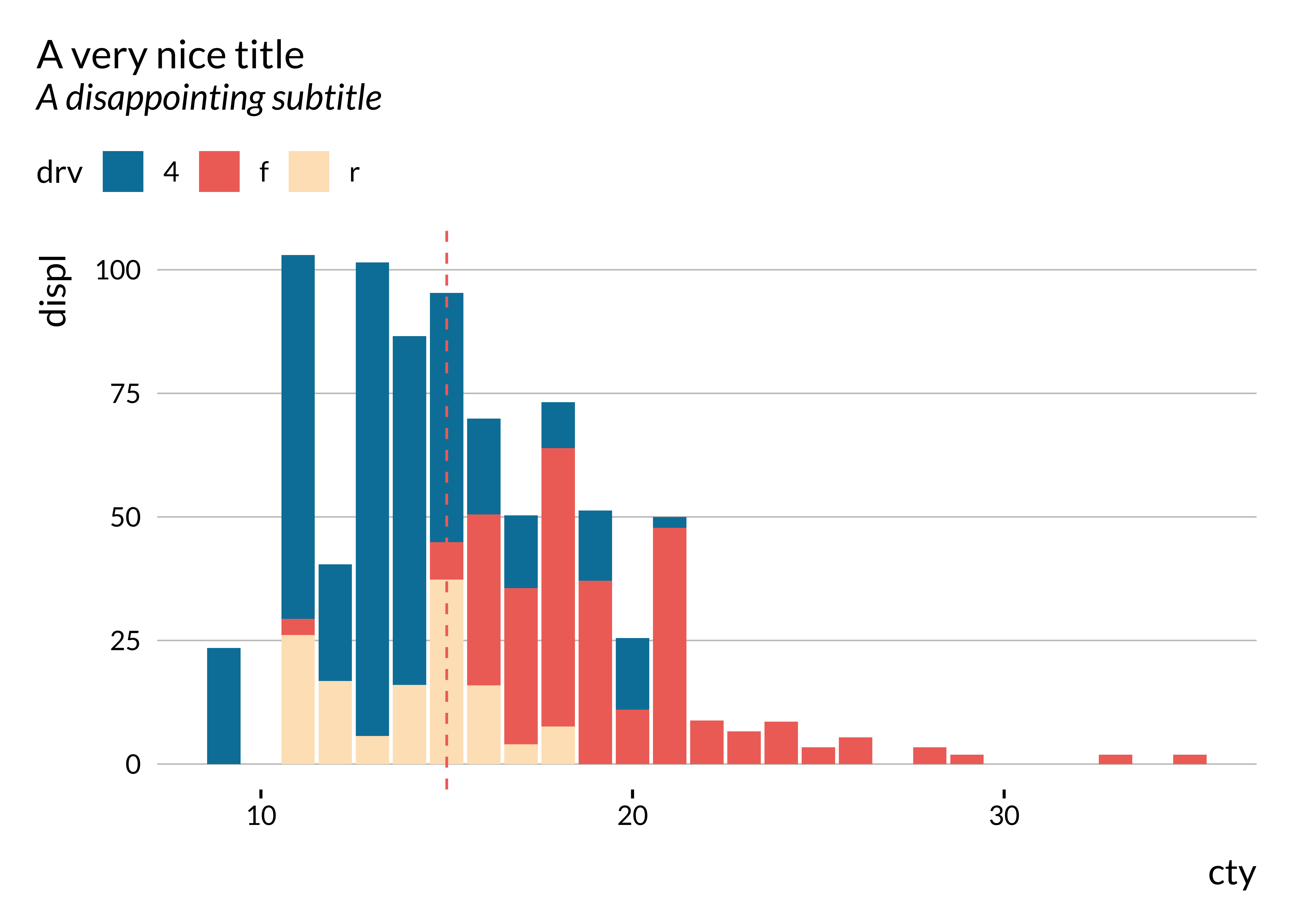
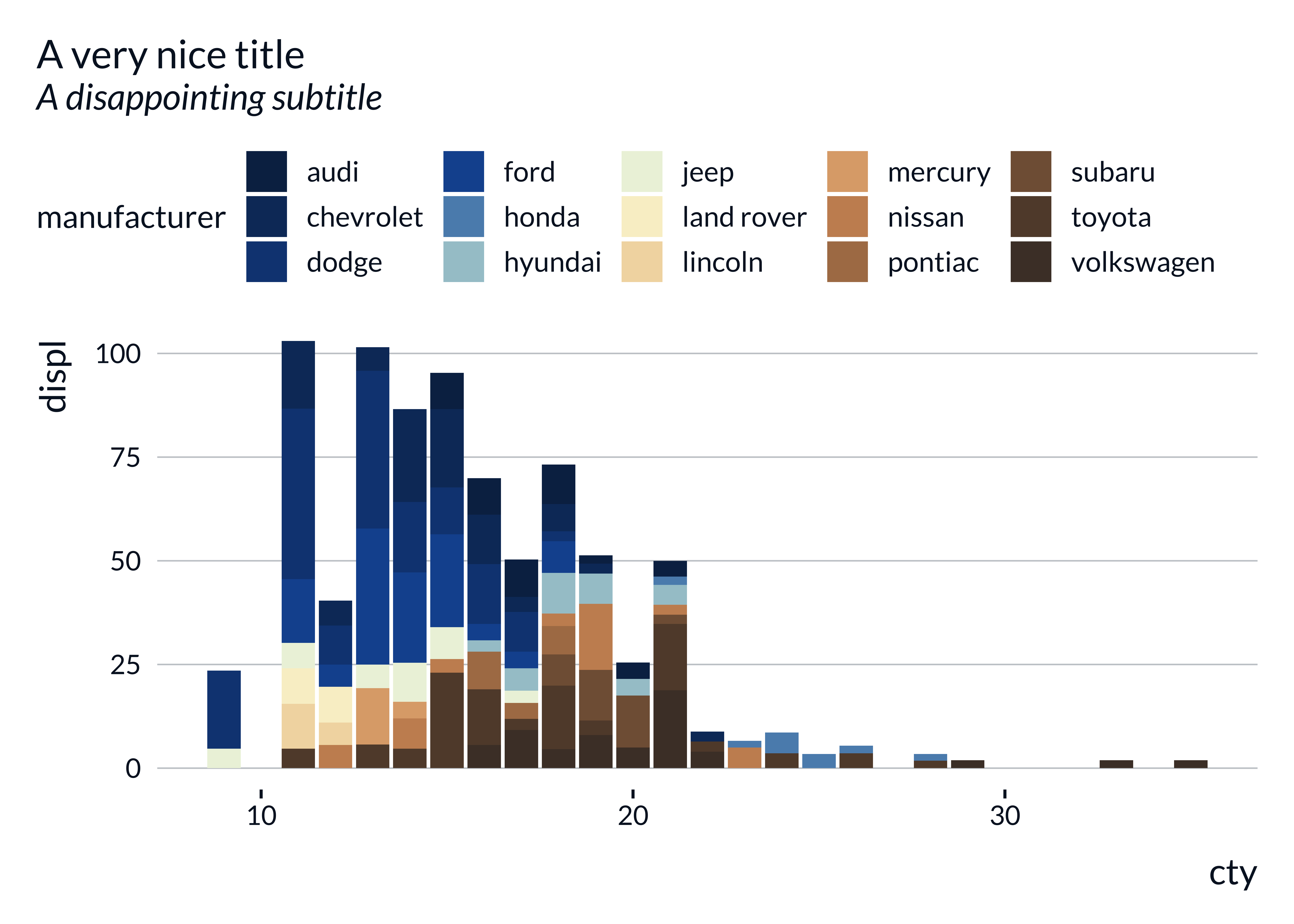
set_mediocre_all() before. The following example
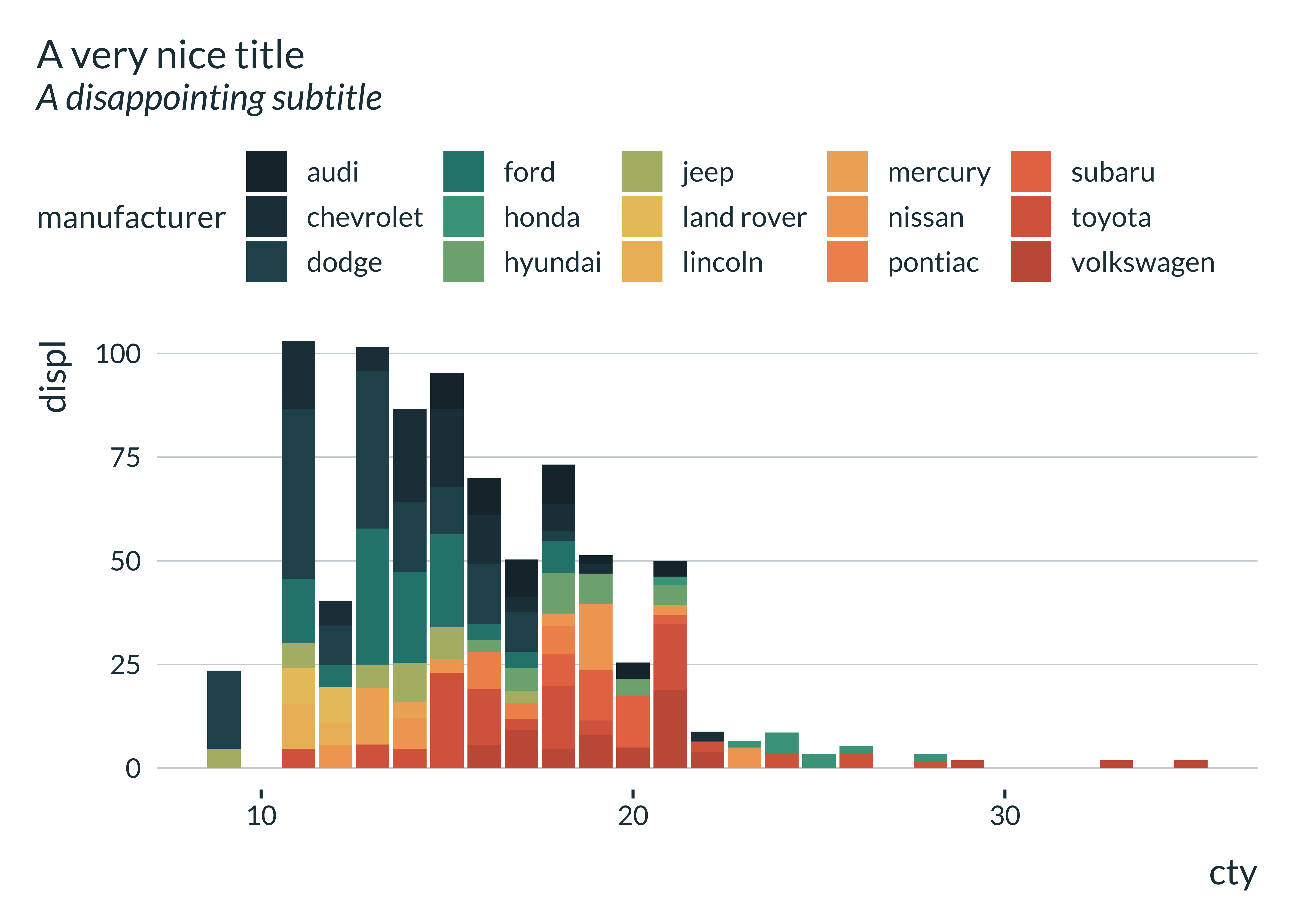
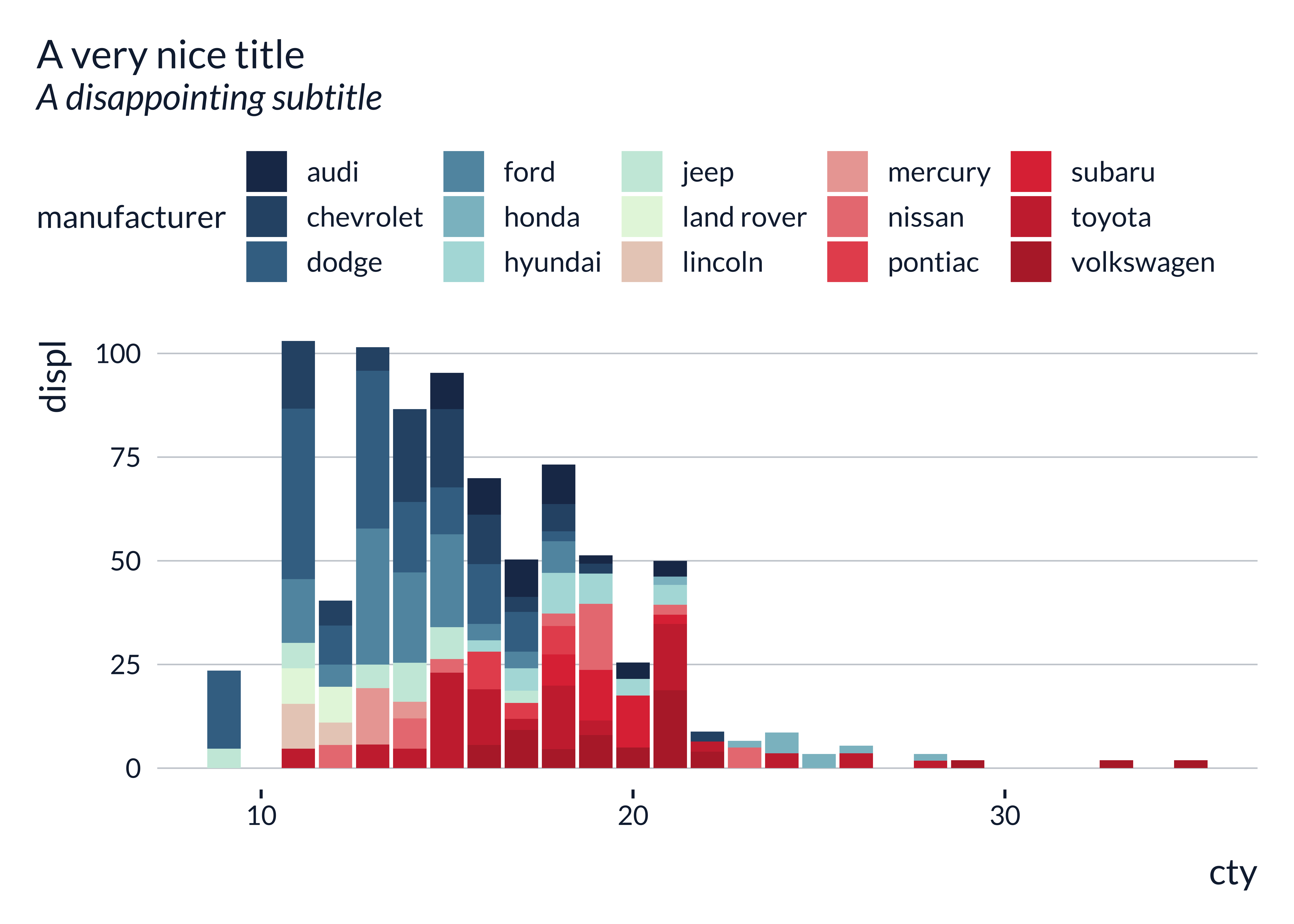
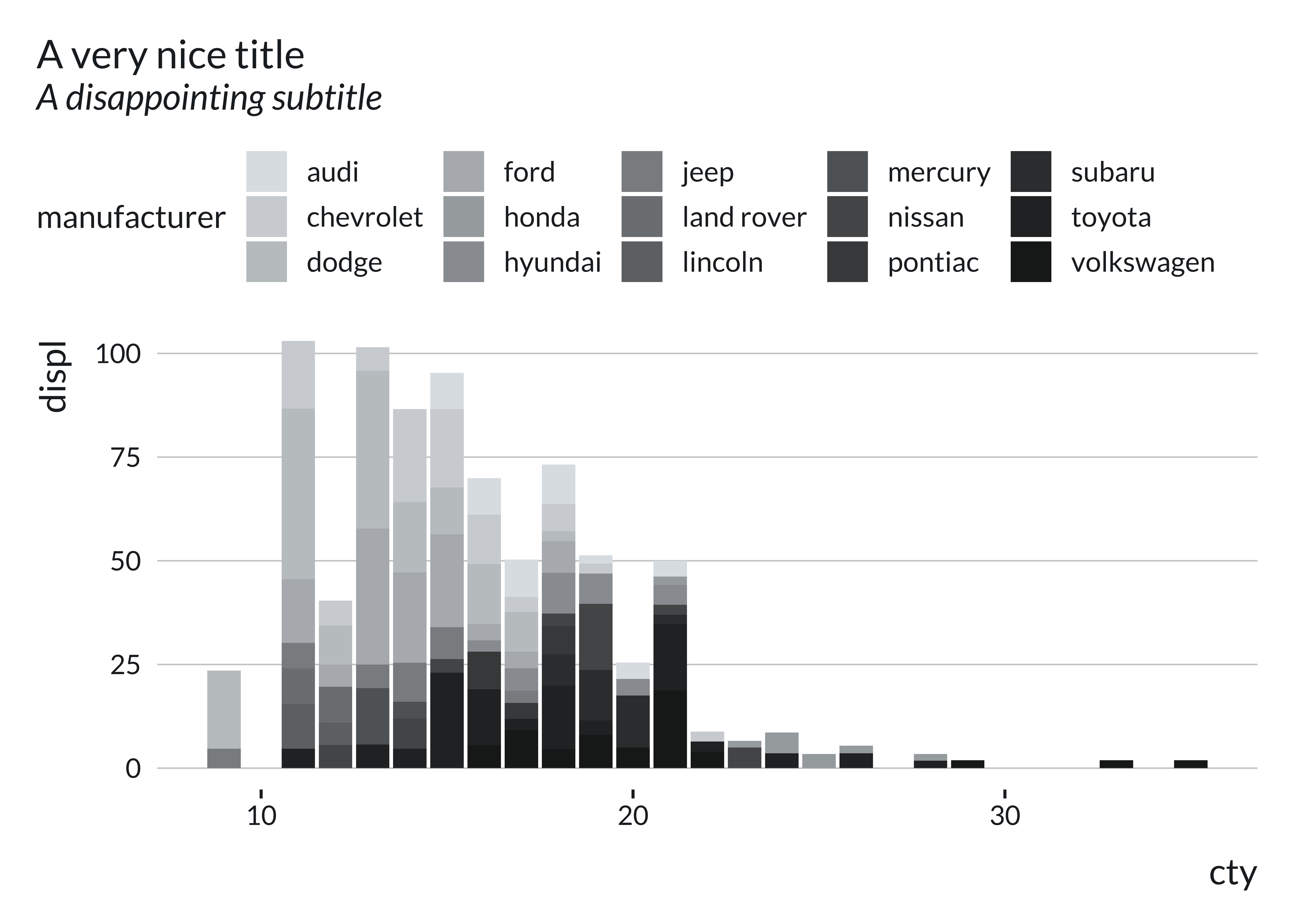
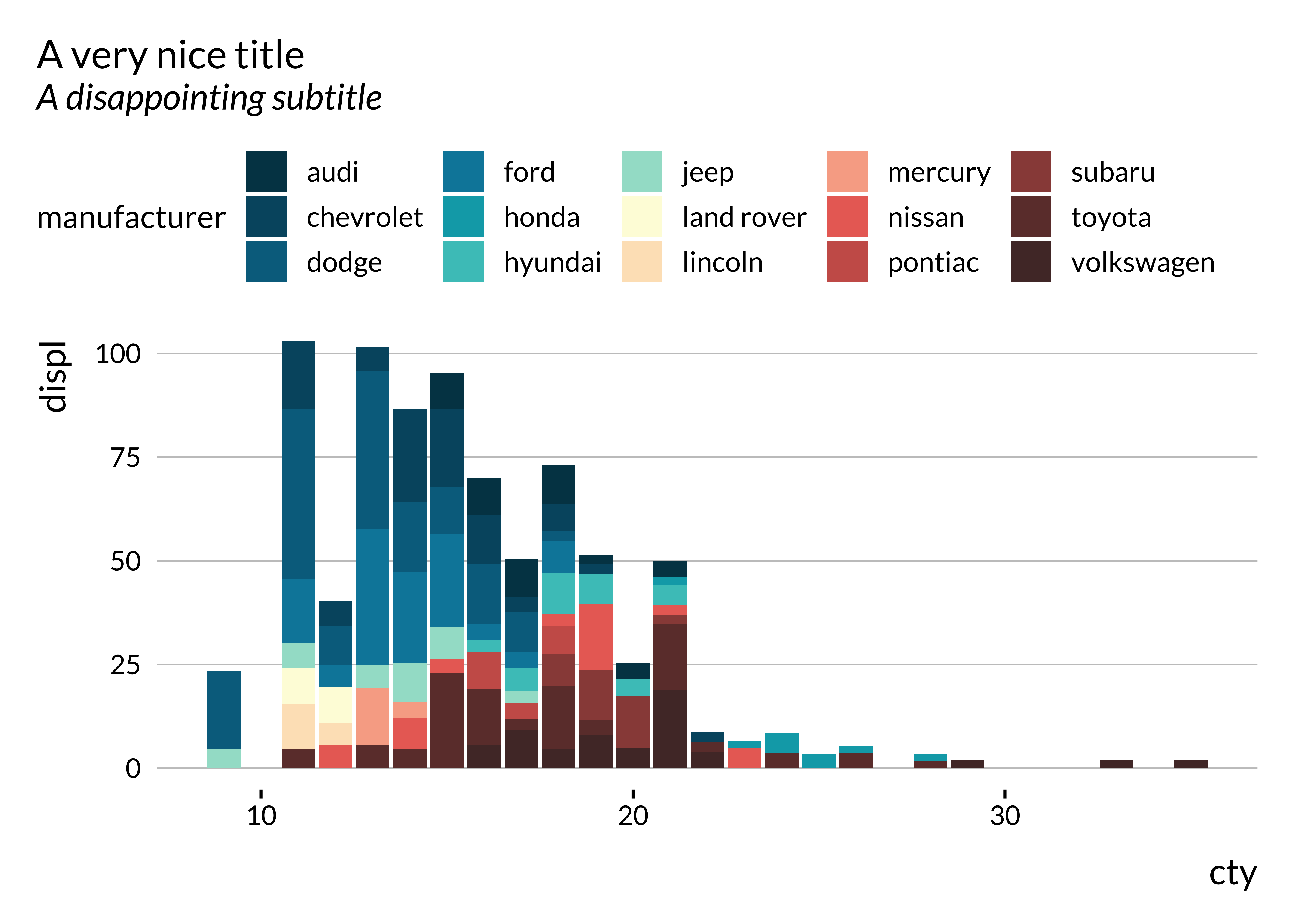
illustrates this feature:
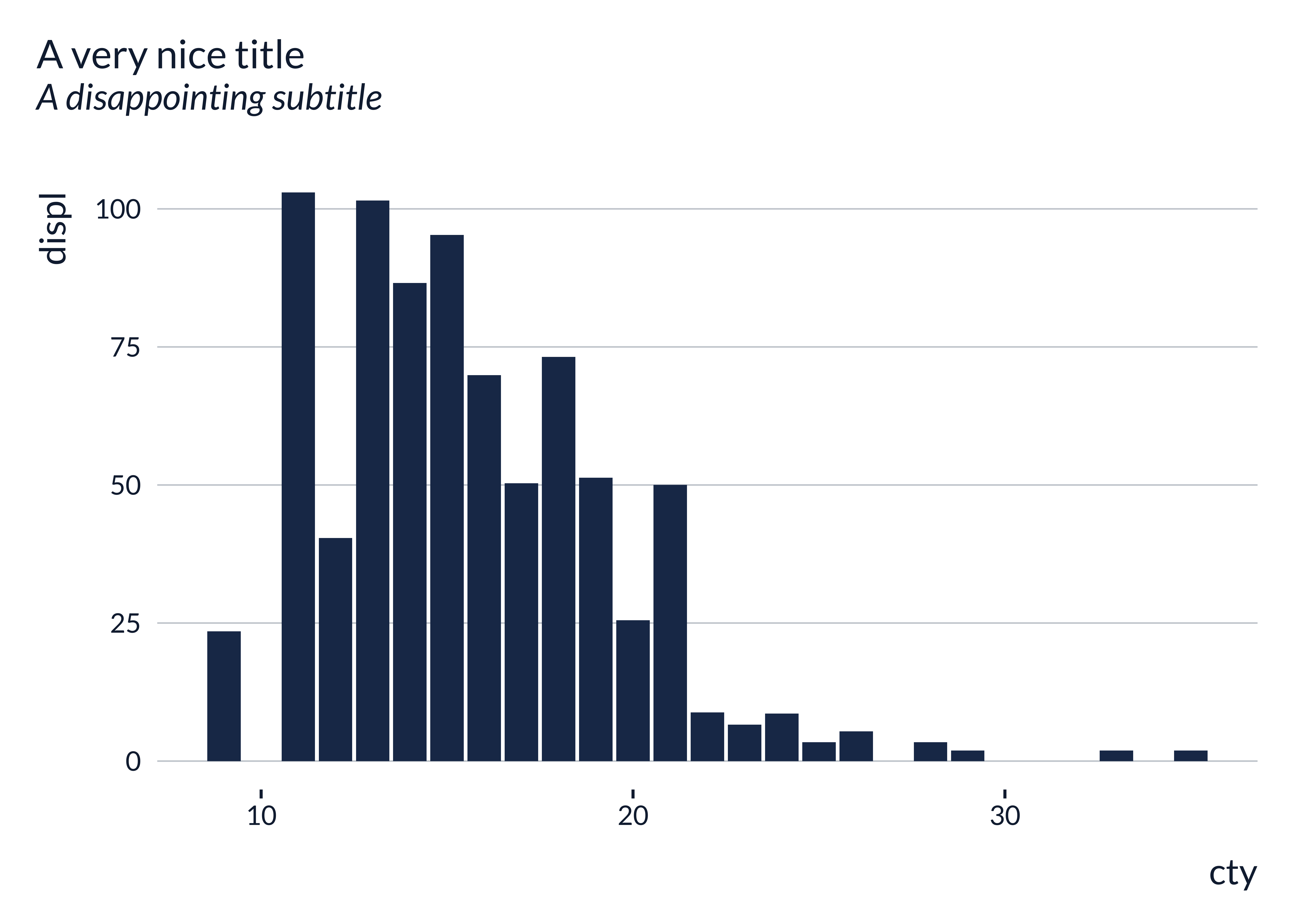
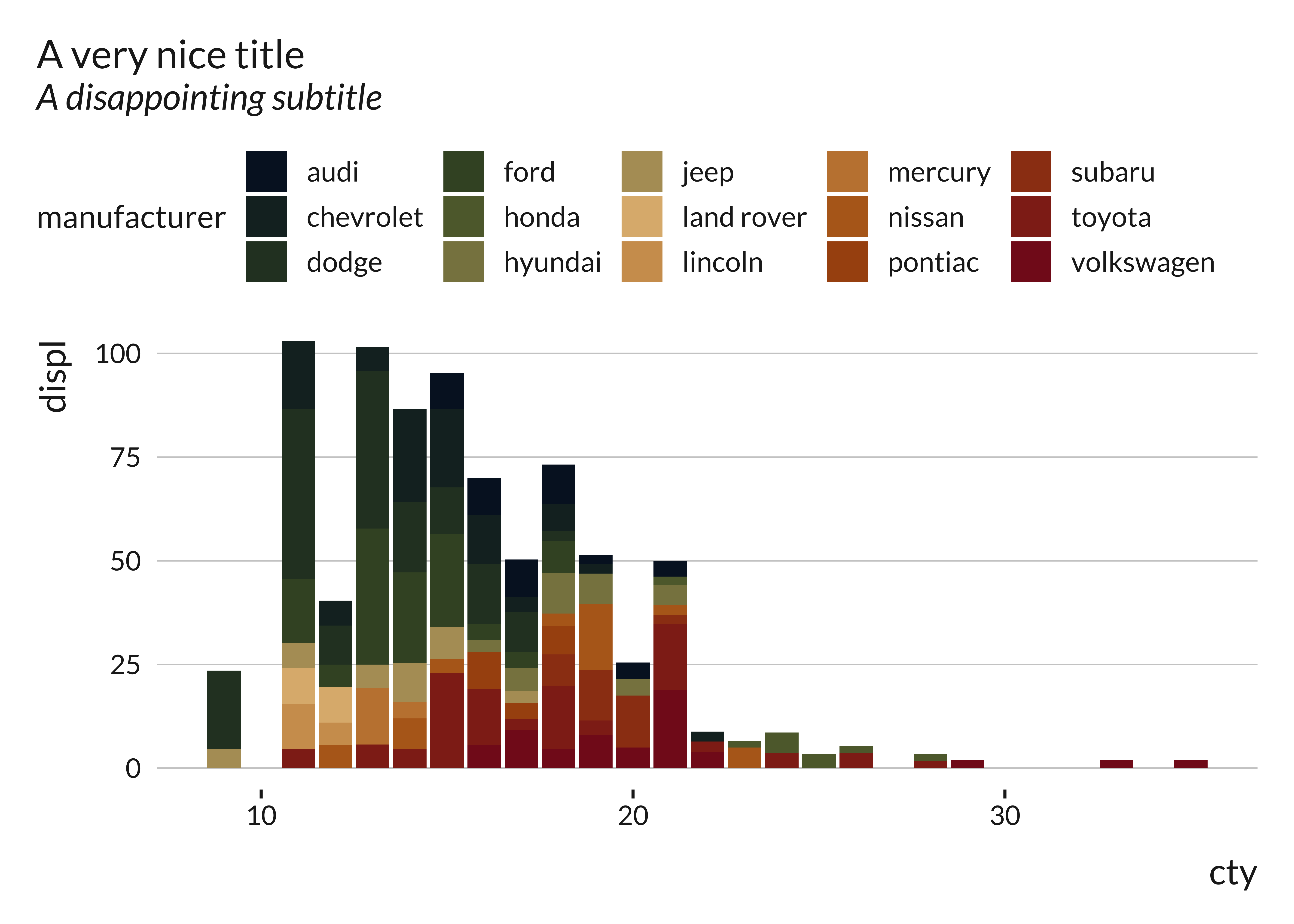
set_mediocre_all()

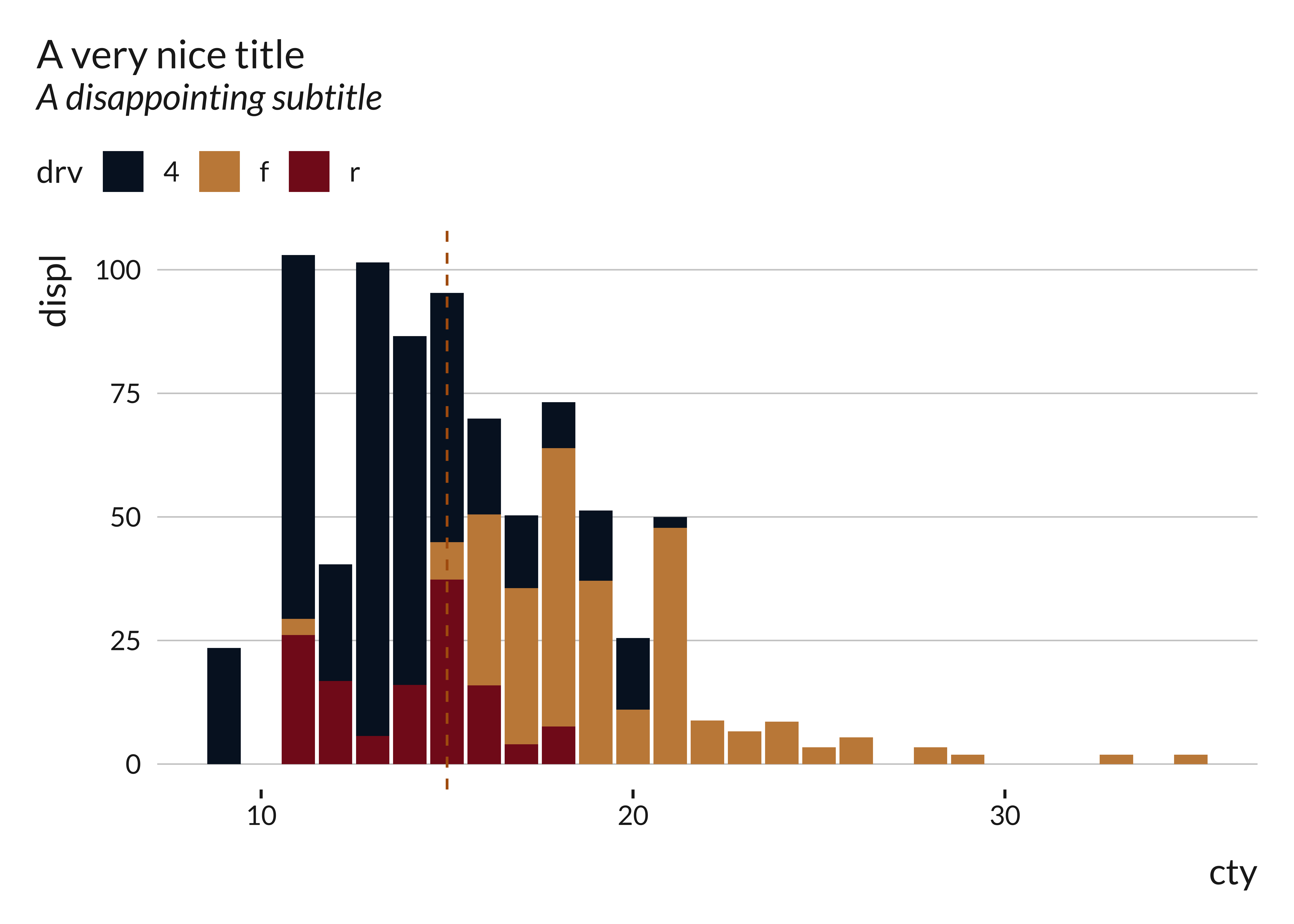
ggplot(data = ggplot2::mpg, aes(x = cty, y = displ, fill = manufacturer)) +
    geom_col() +
    labs(title = "A very nice title", subtitle = "A disappointing subtitle")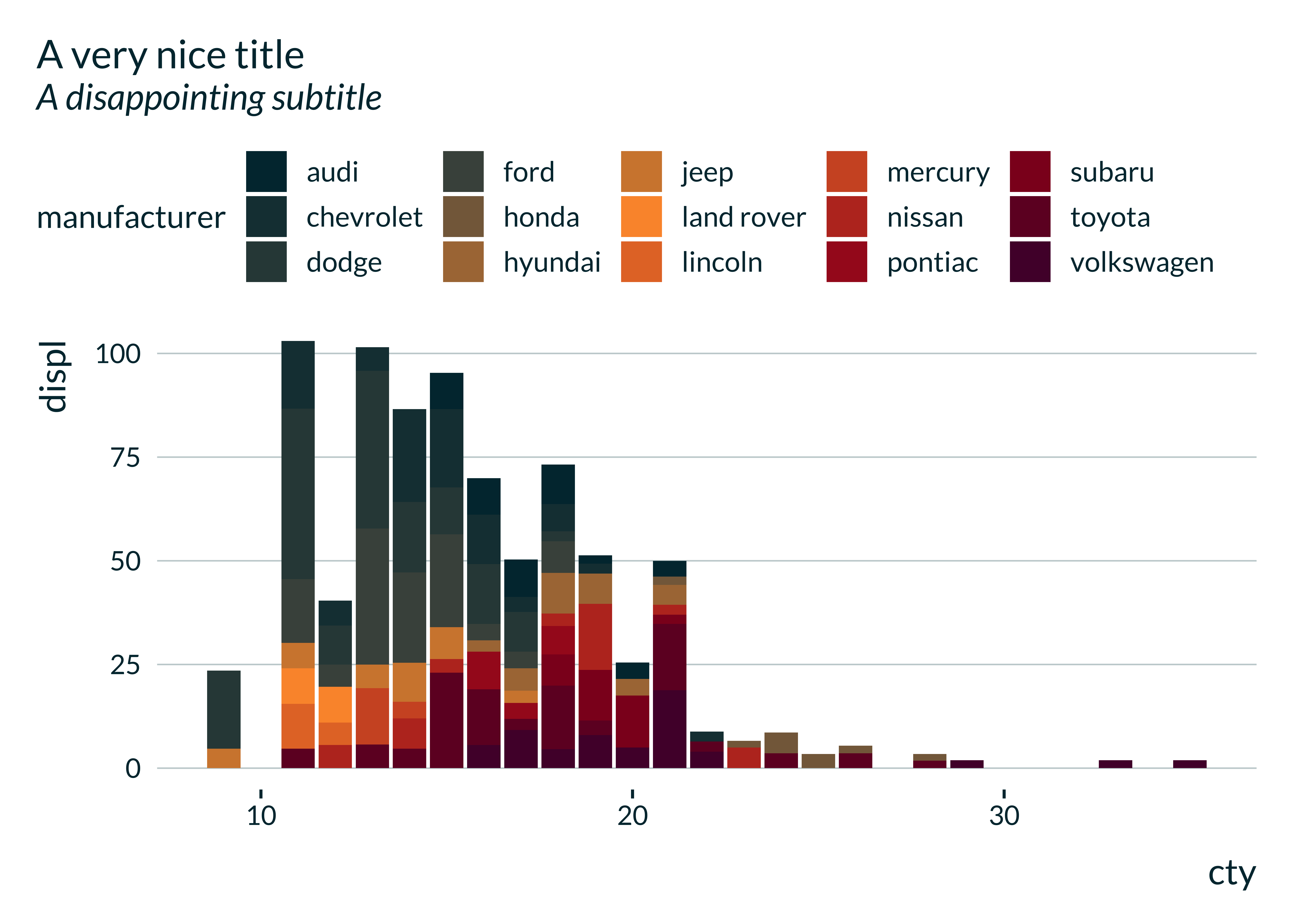
The function set_mediocre_all takes several arguments:
pal, background, second_pair and
gradient along with the usual base_size,
base_family, base_line_size and
base_rect_size. The following subsections describe the use
of the three first arguments.
Changing the palette
Available palettes are: autumn, rainbow, green, hotcold,
blackandwhite, coty, leo, portal, pem. A palette defines the color of
the theme and the color scale used in the graphs, ie the color
of the axes and text for the theme and the colors used in the legend for
the color scale. To change the palette to “coty” for instance, just set
the argument pal equal to “coty” when calling the function
set_mediocre_all at the beginning of the document. All
subsequent graphs will be created using similar code, the only
difference is the name of the palette in
set_mediocre_all
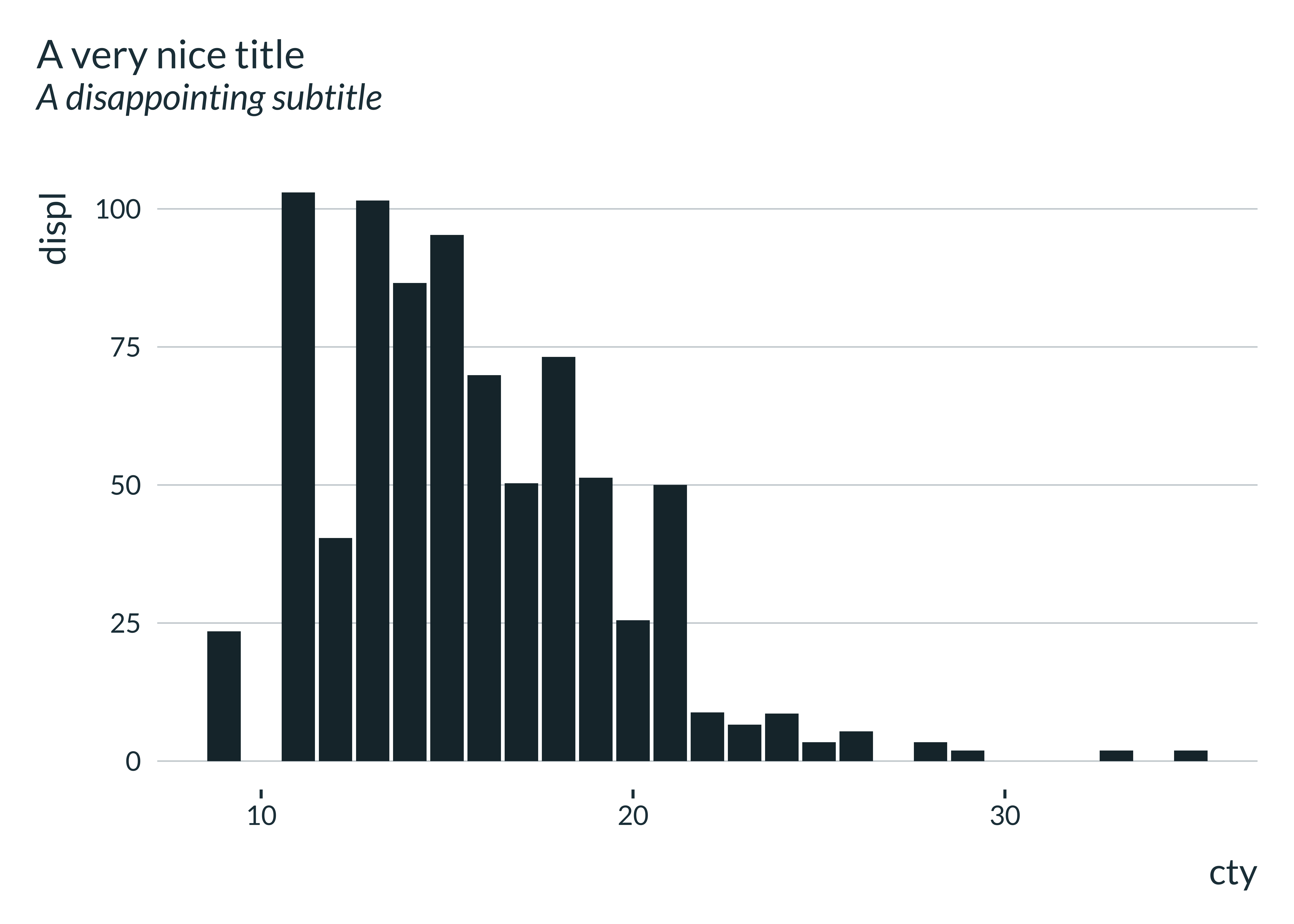
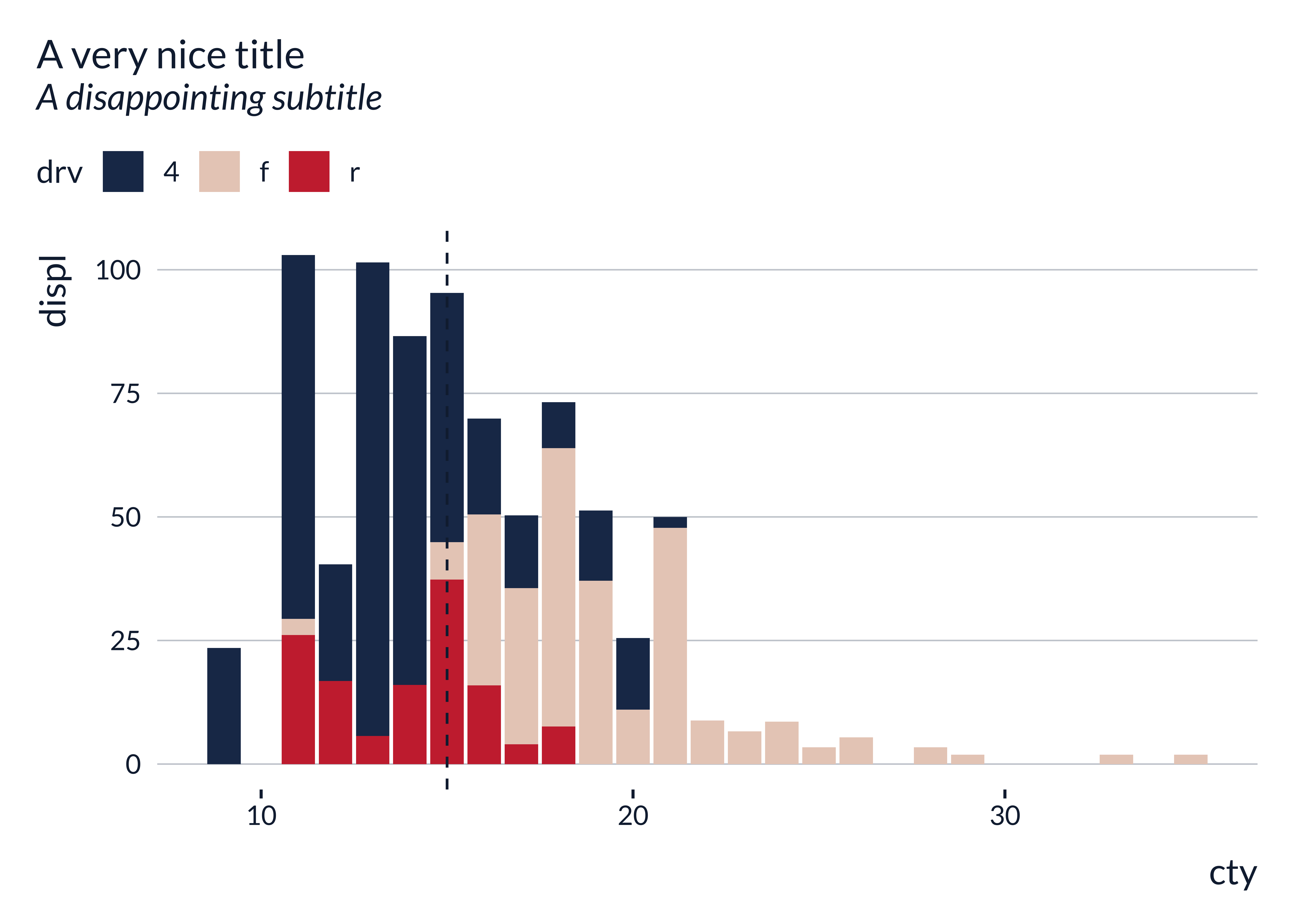
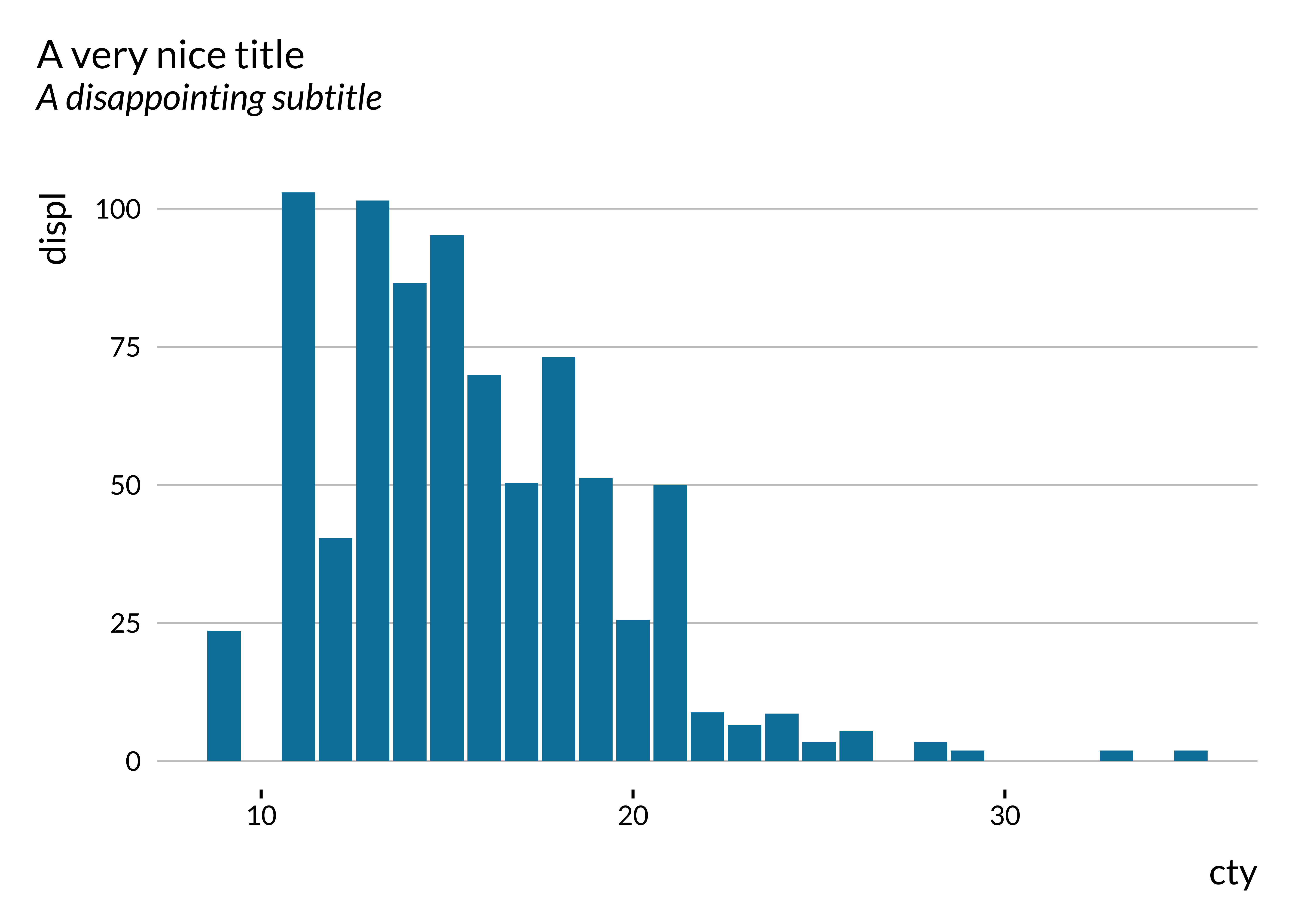
set_mediocre_all(pal = "coty")

ggplot(data = ggplot2::mpg, aes(x = cty, y = displ, fill = manufacturer)) +
    geom_col() +
    labs(title = "A very nice title", subtitle = "A disappointing subtitle")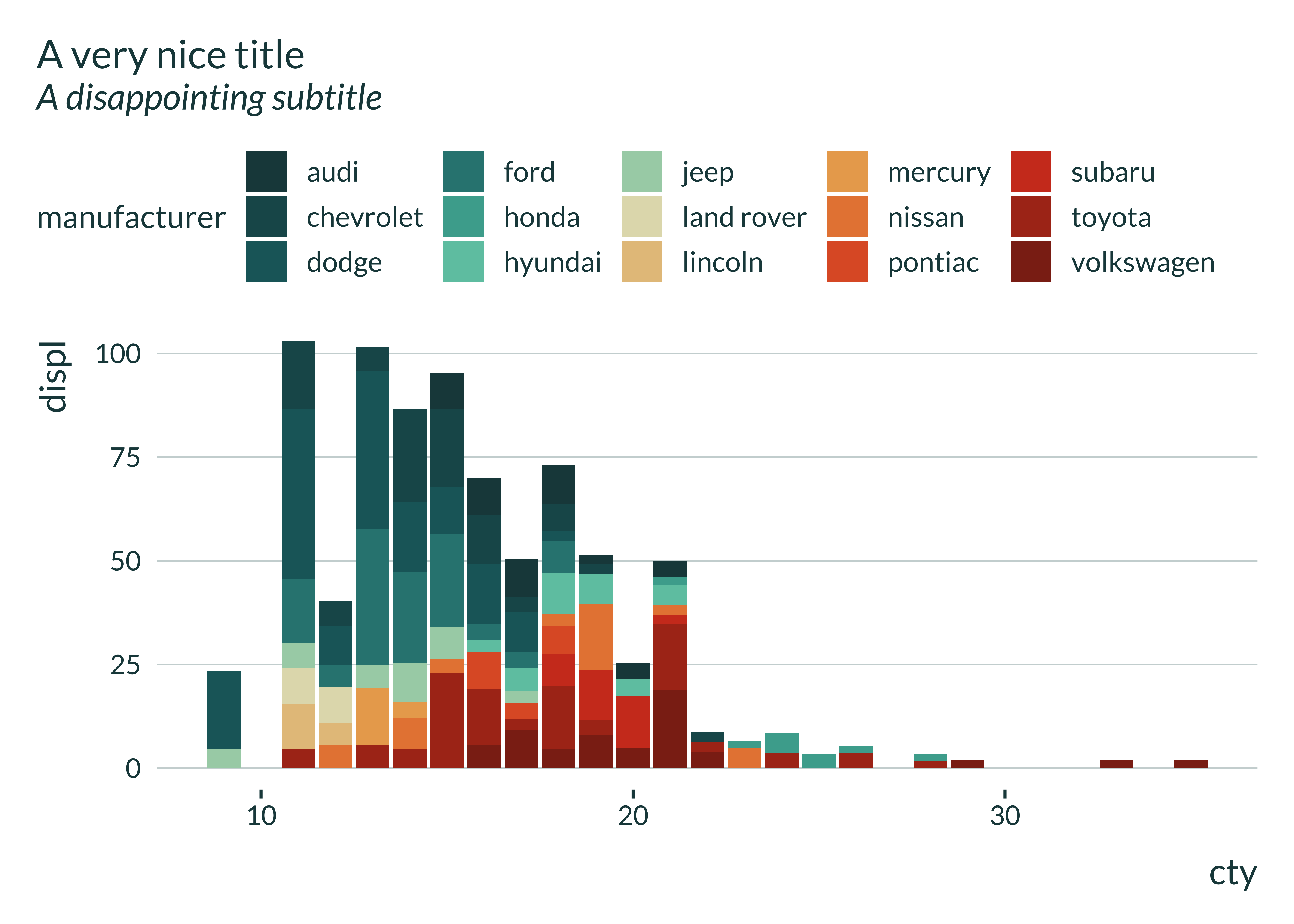
coty
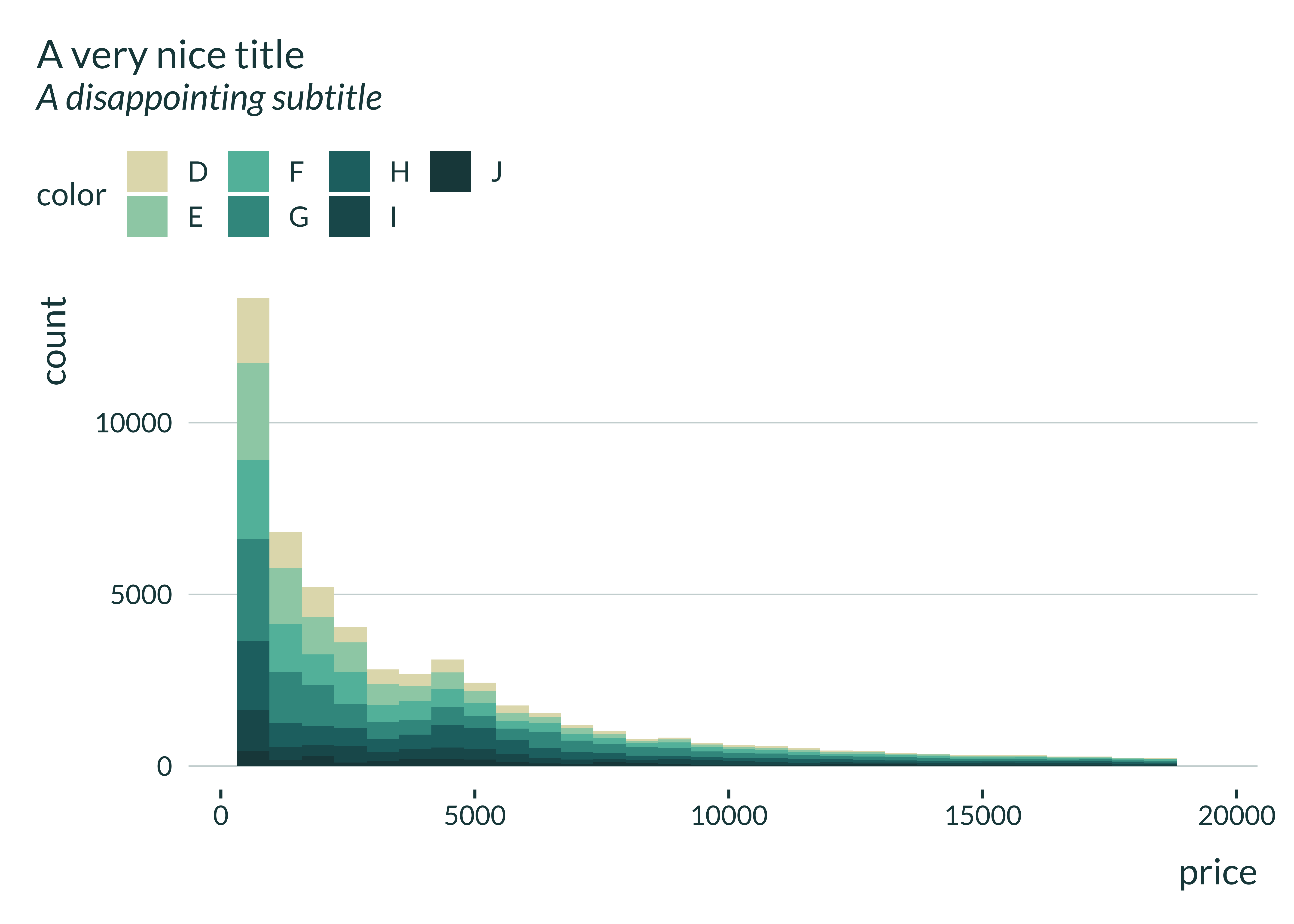
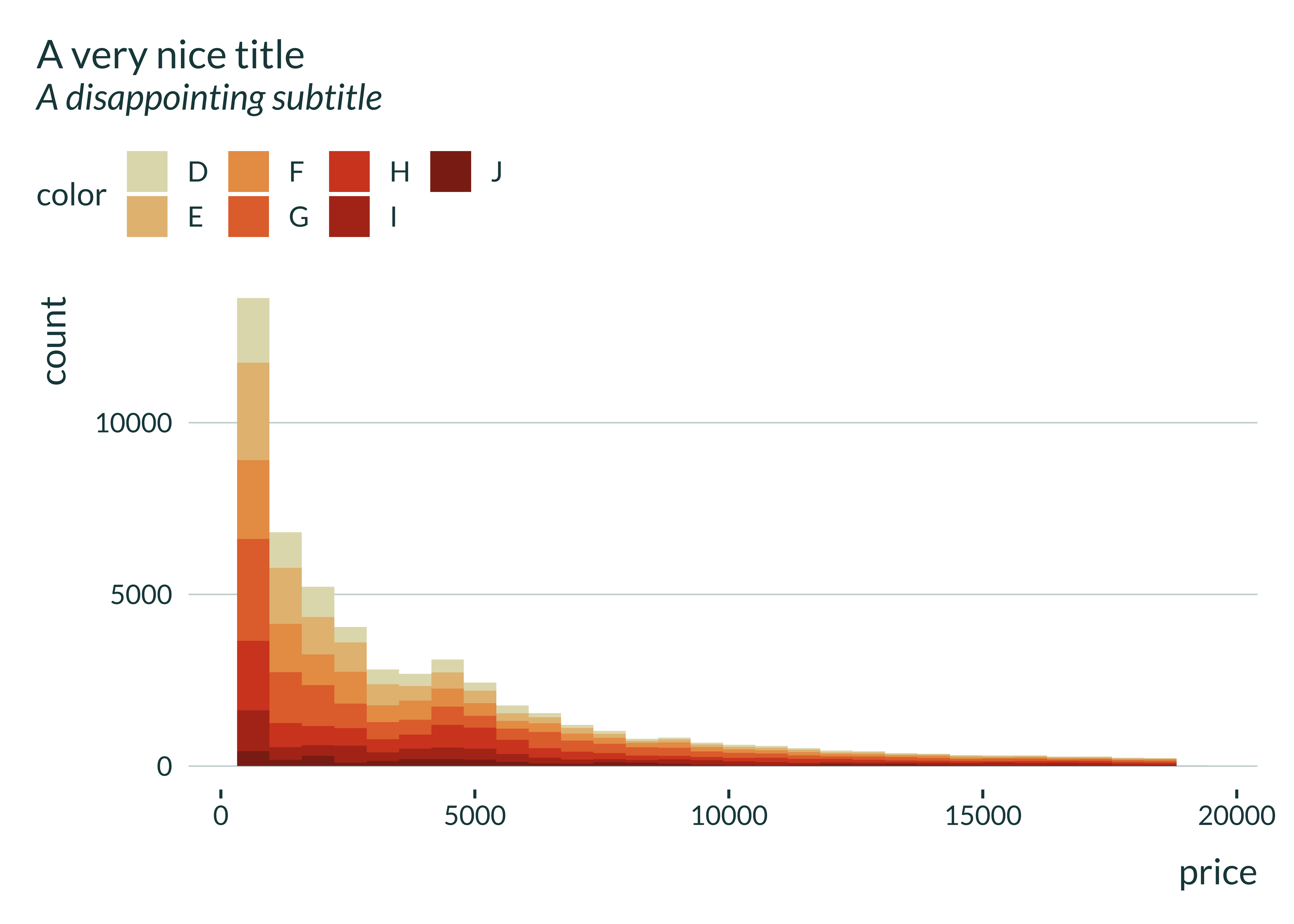
A (tentatively) colorblind friendly palette, based on a NPR map.


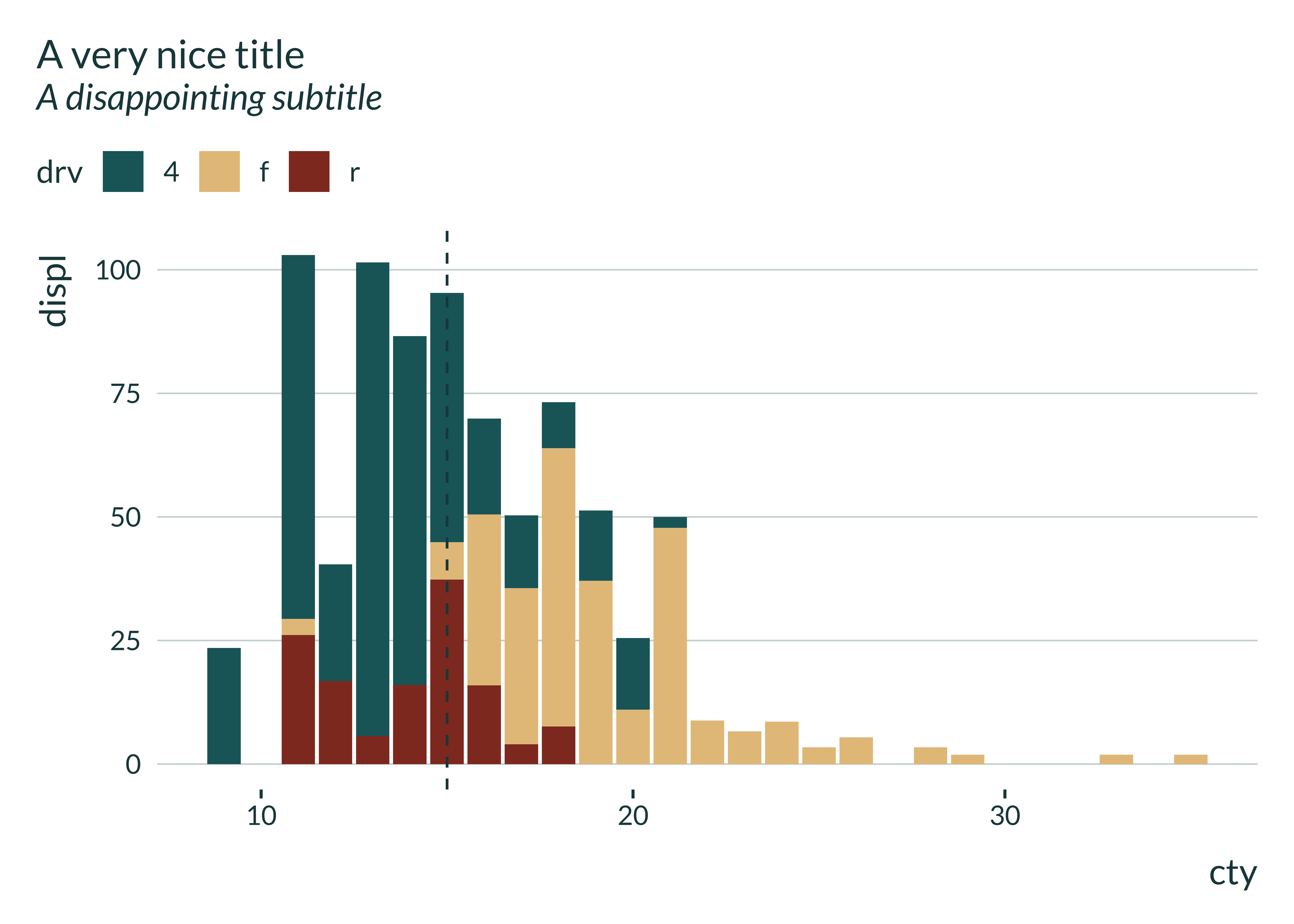
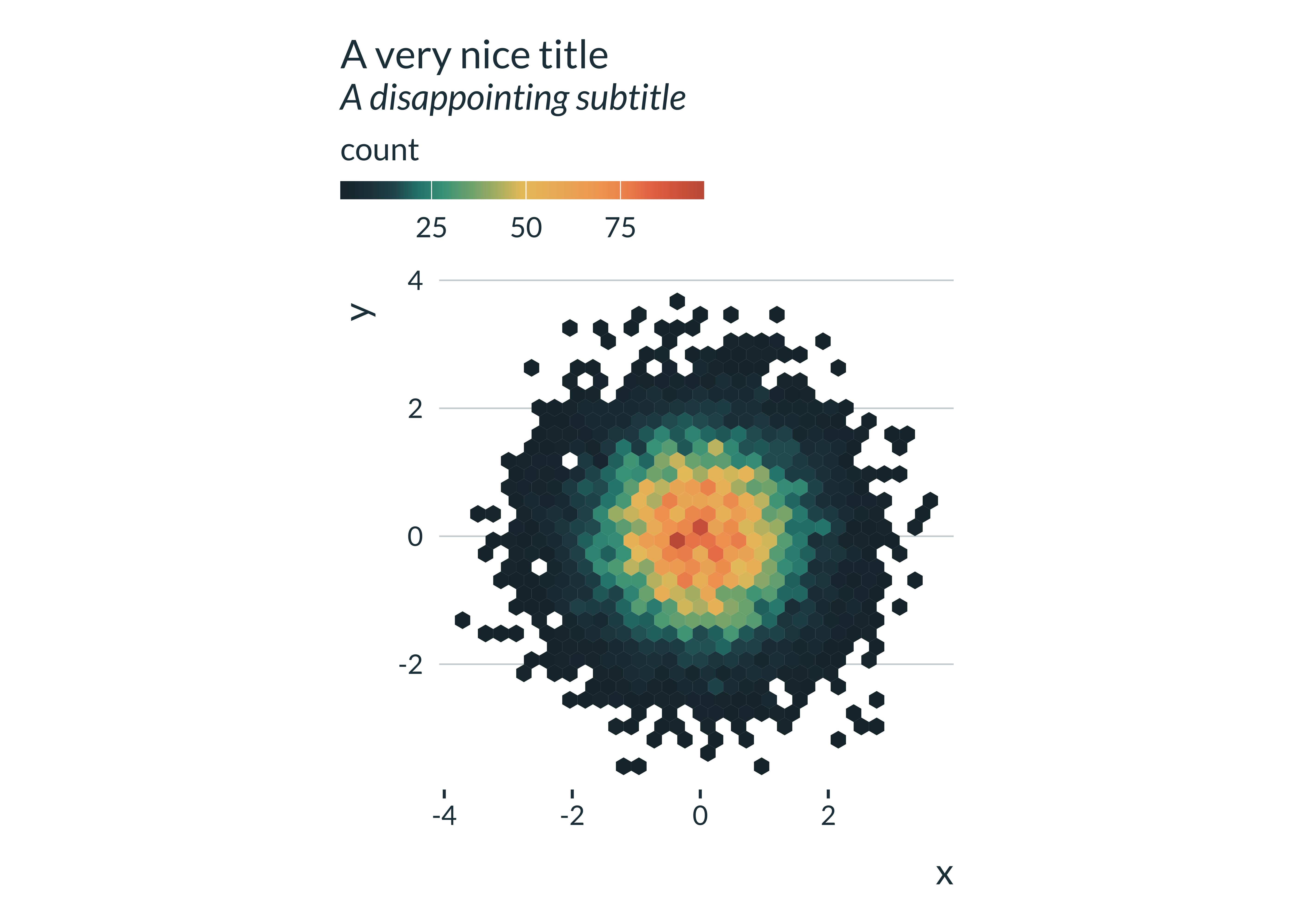
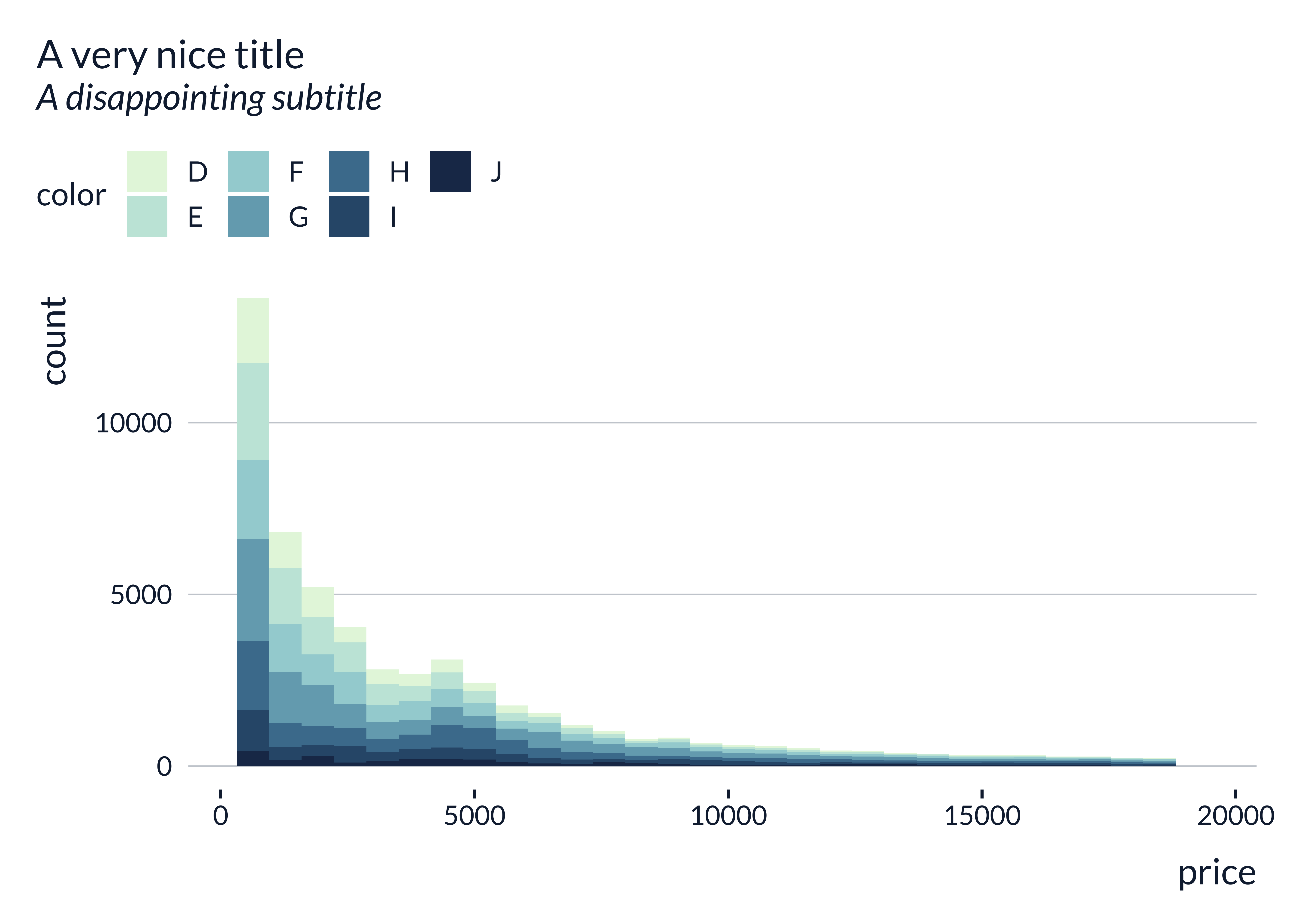
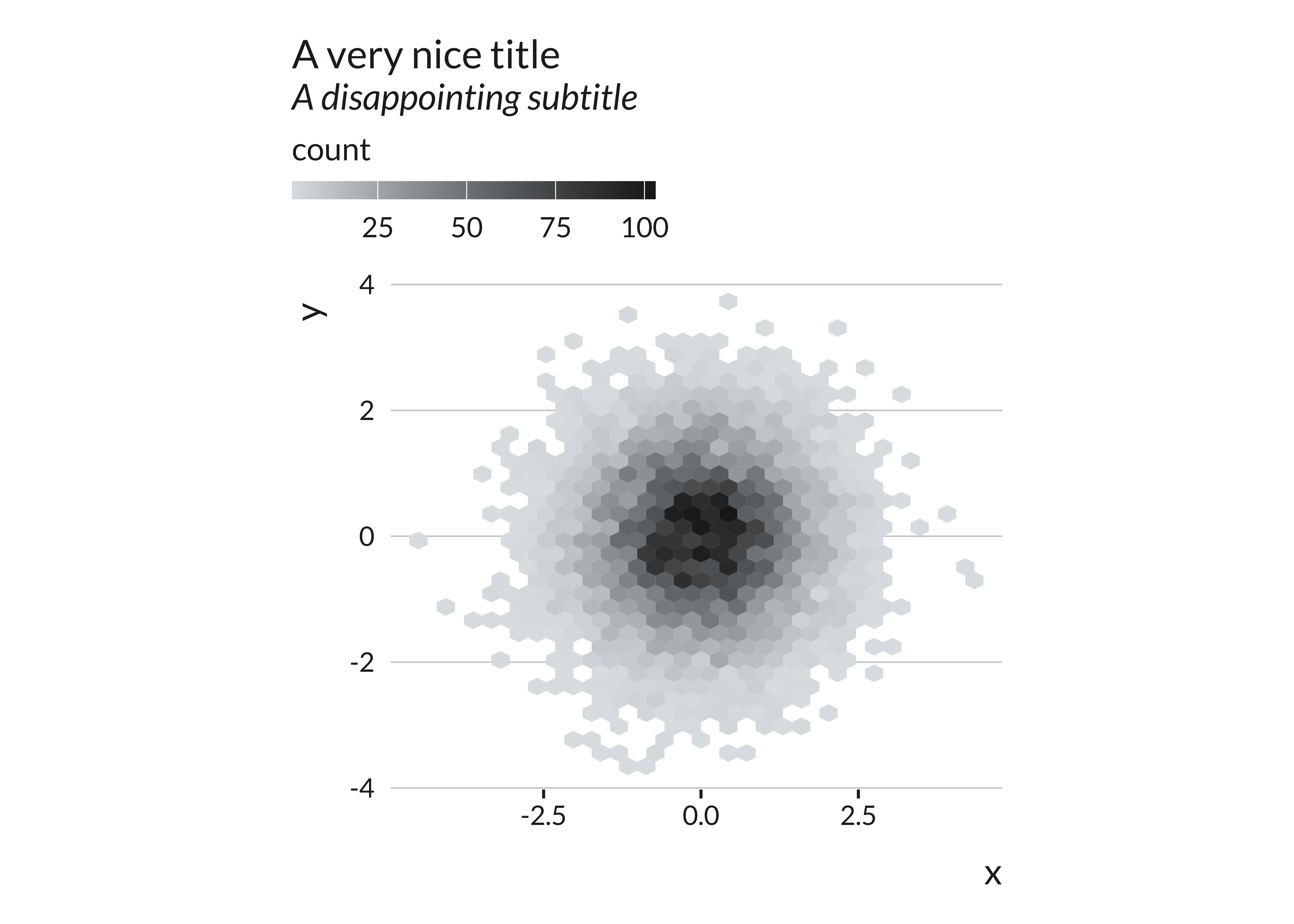
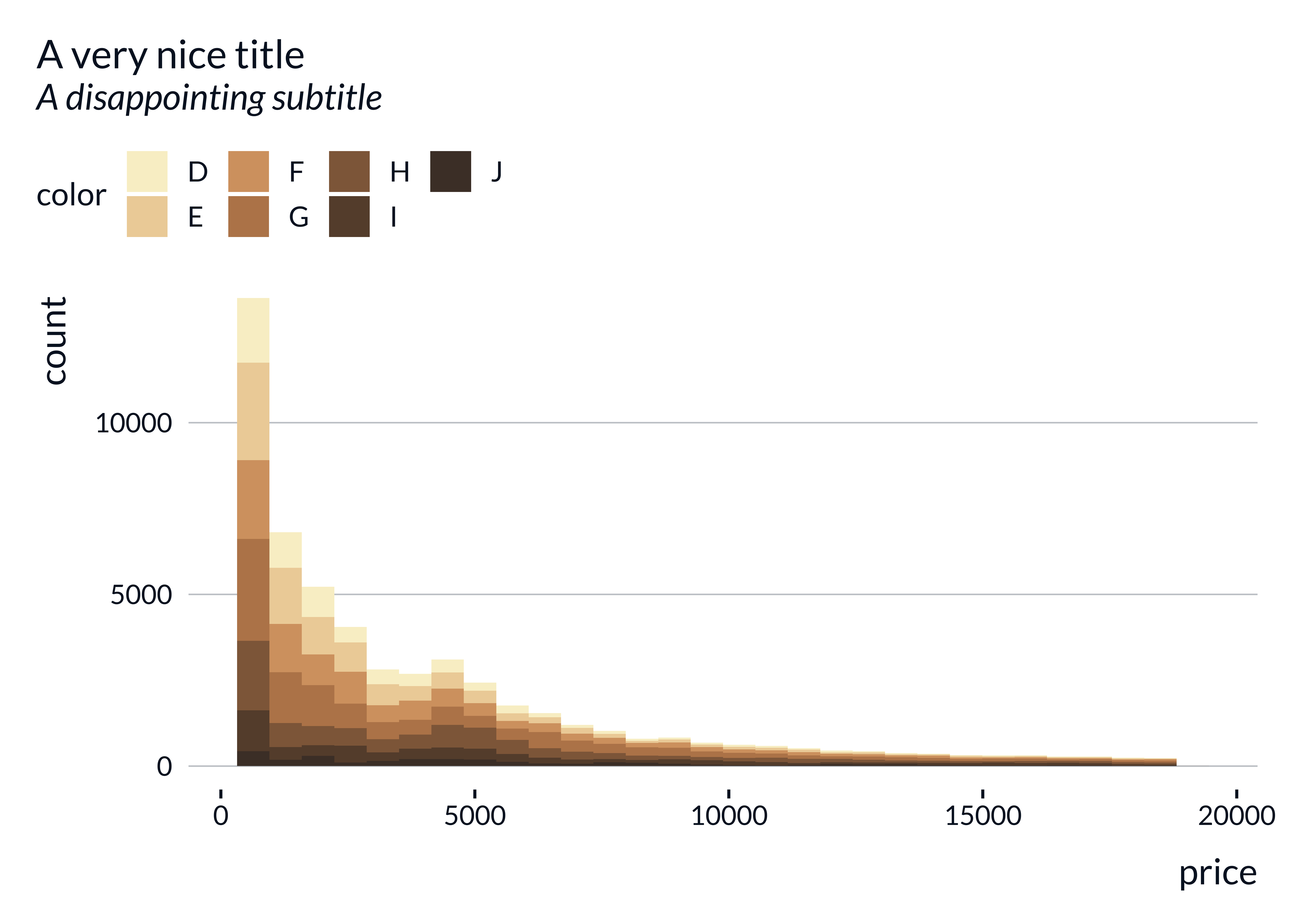
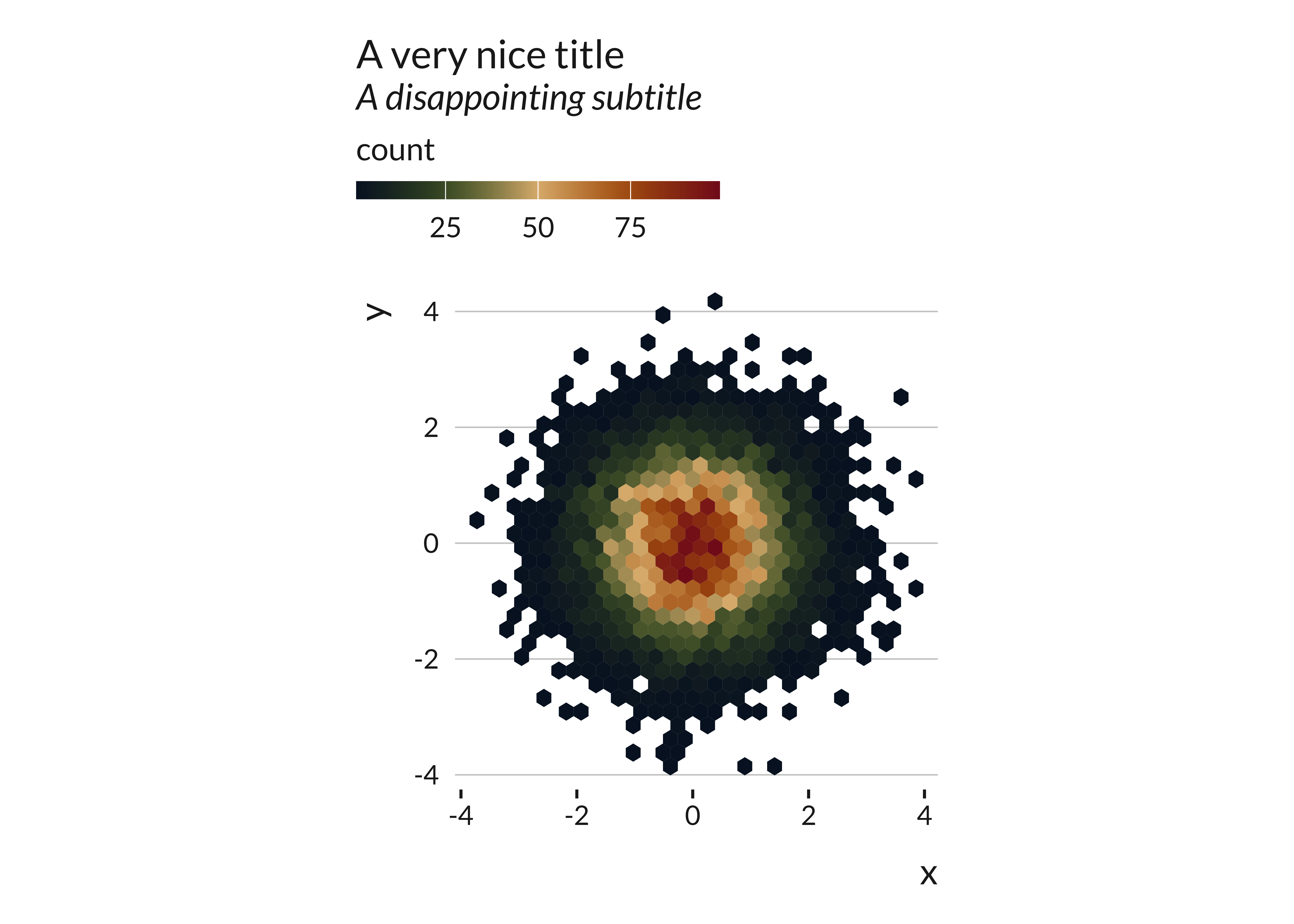
#> `stat_bin2d()` using `bins = 30`. Pick better value `binwidth`.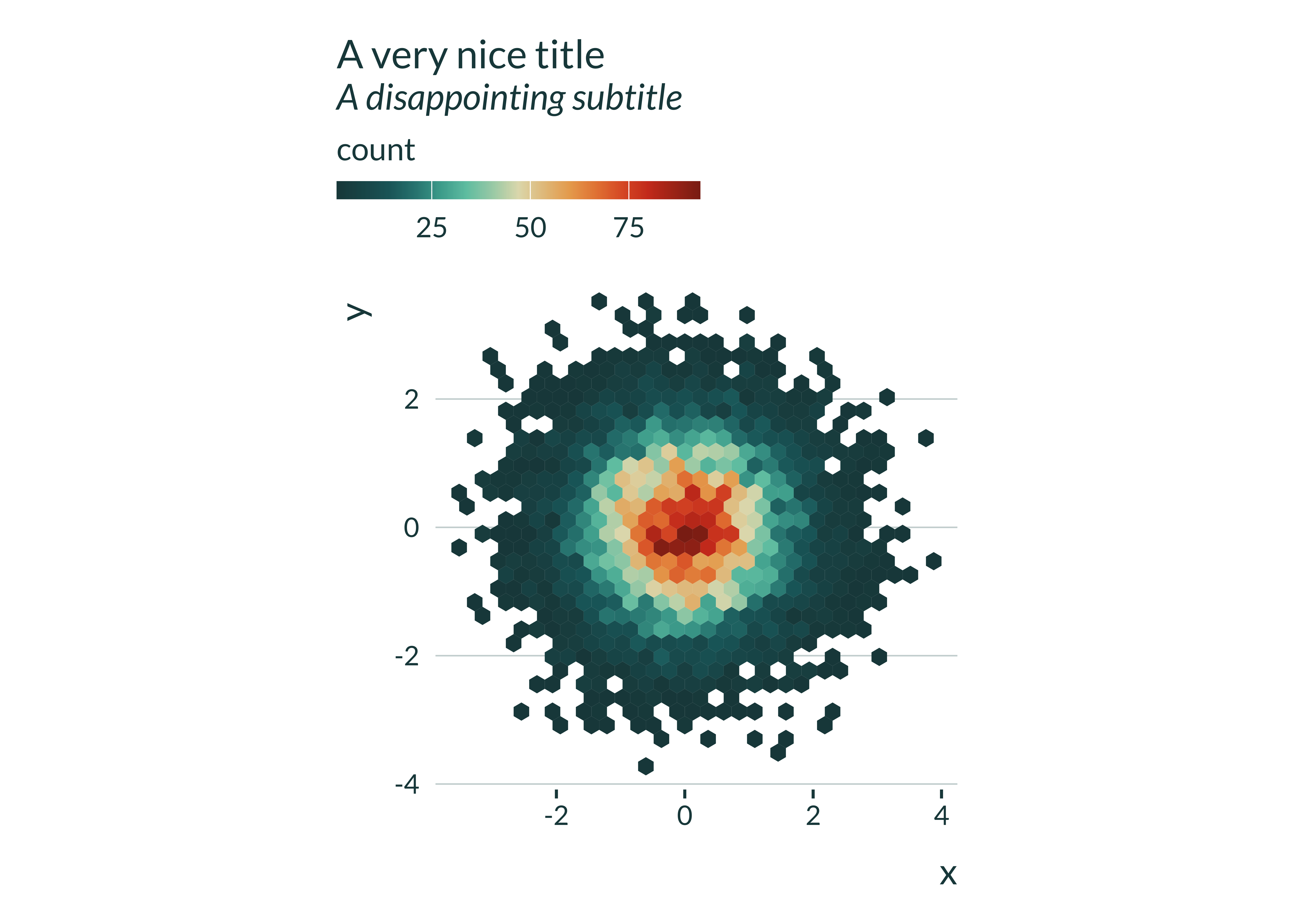
Using a gradient palette
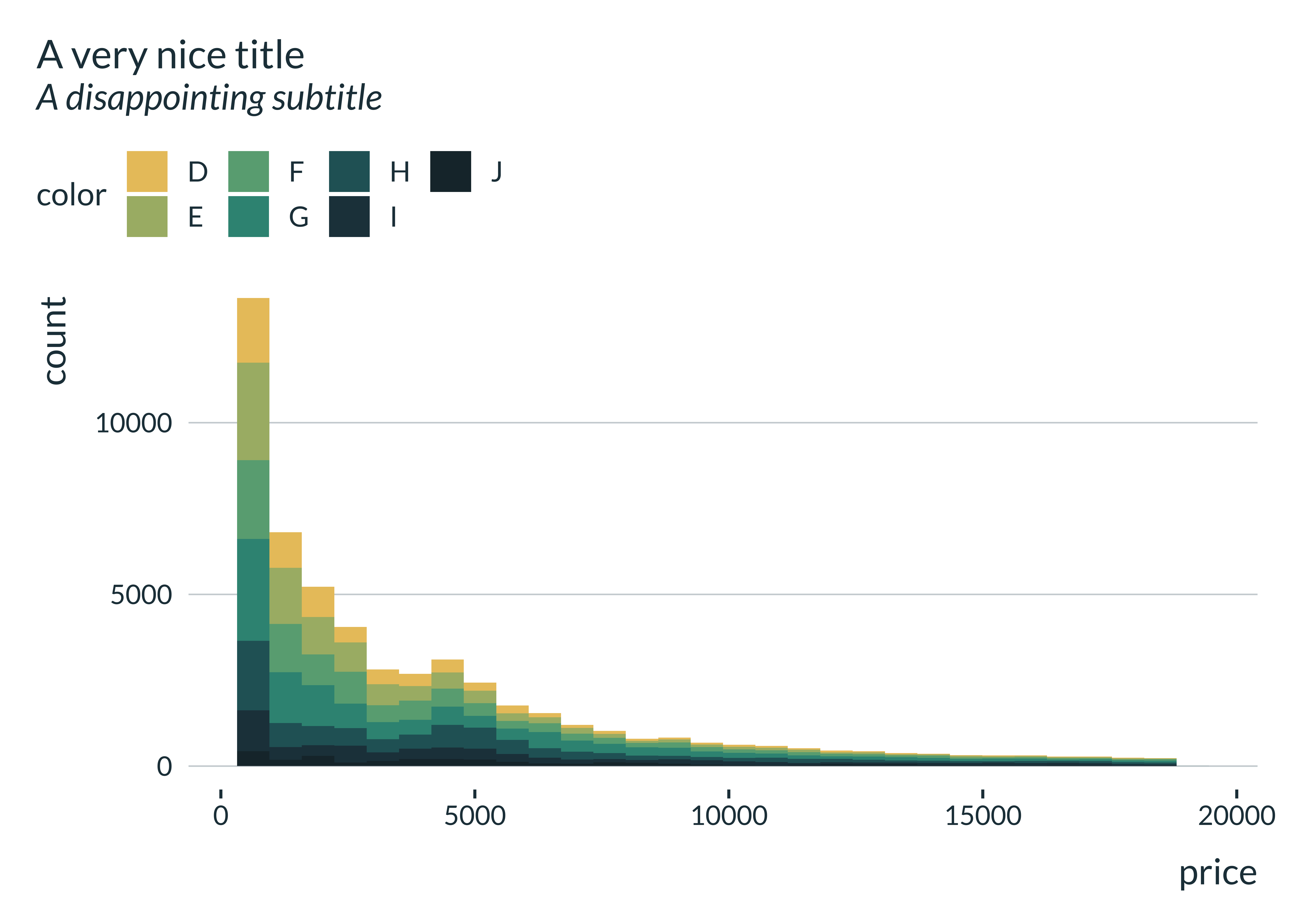
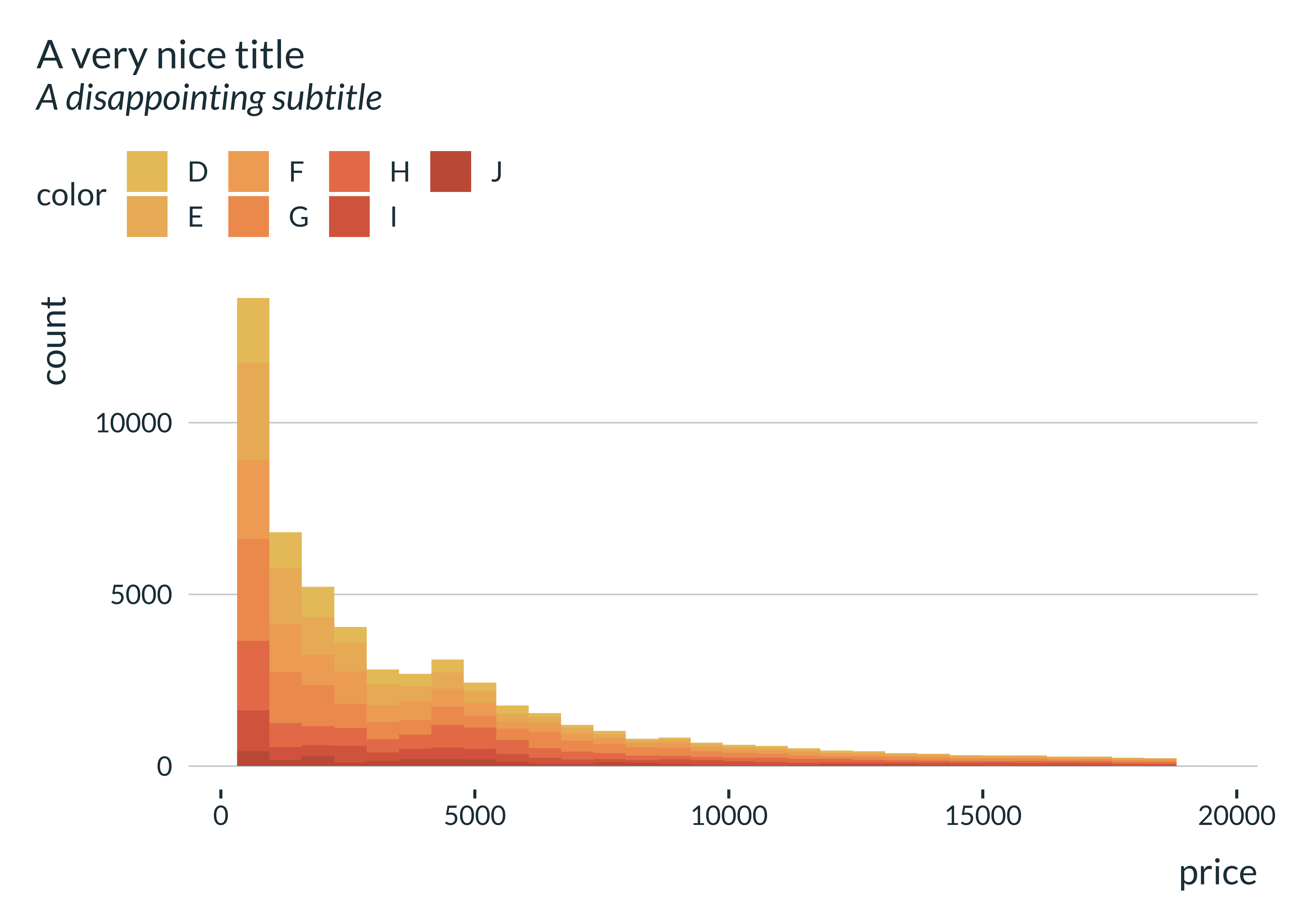
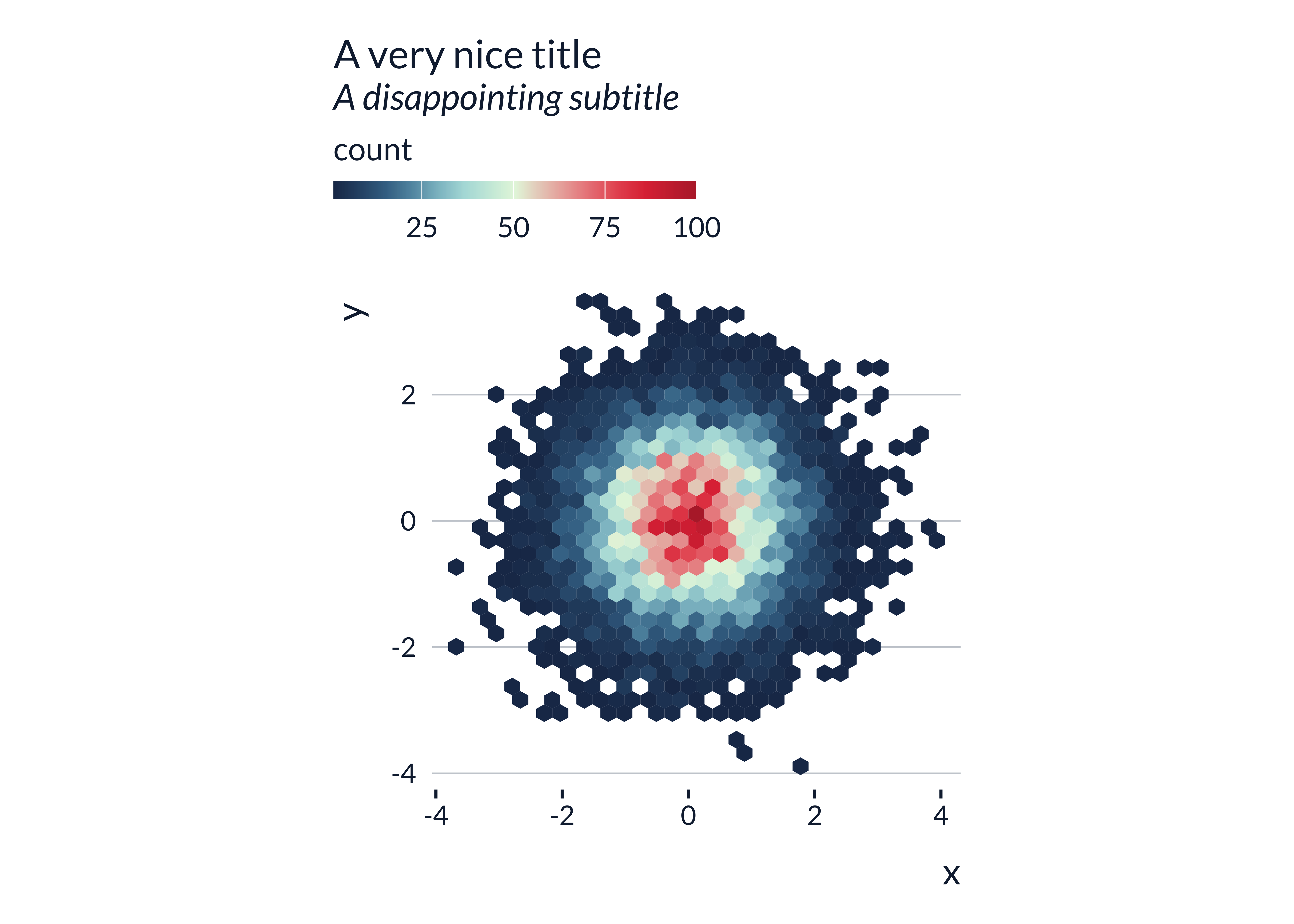
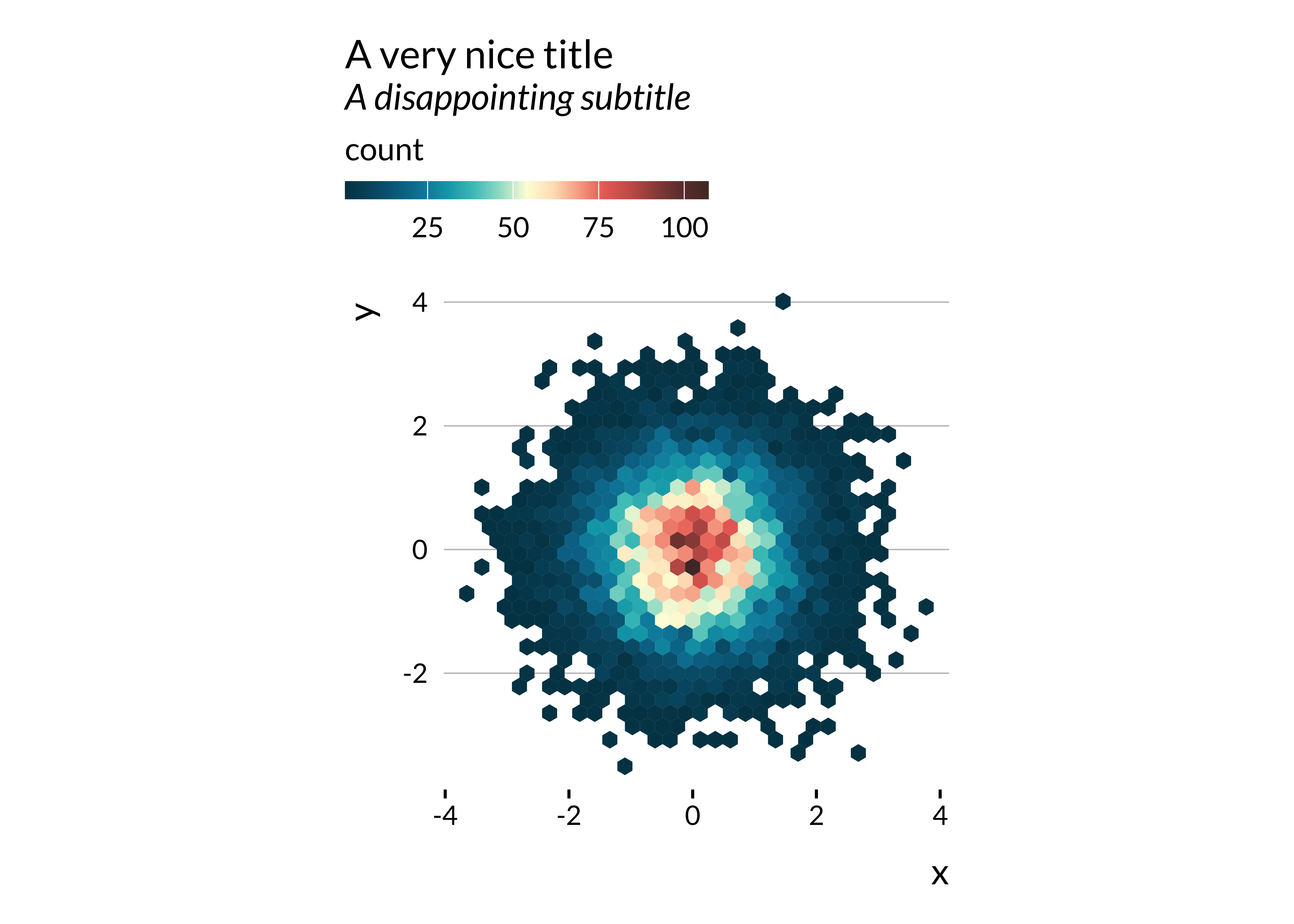
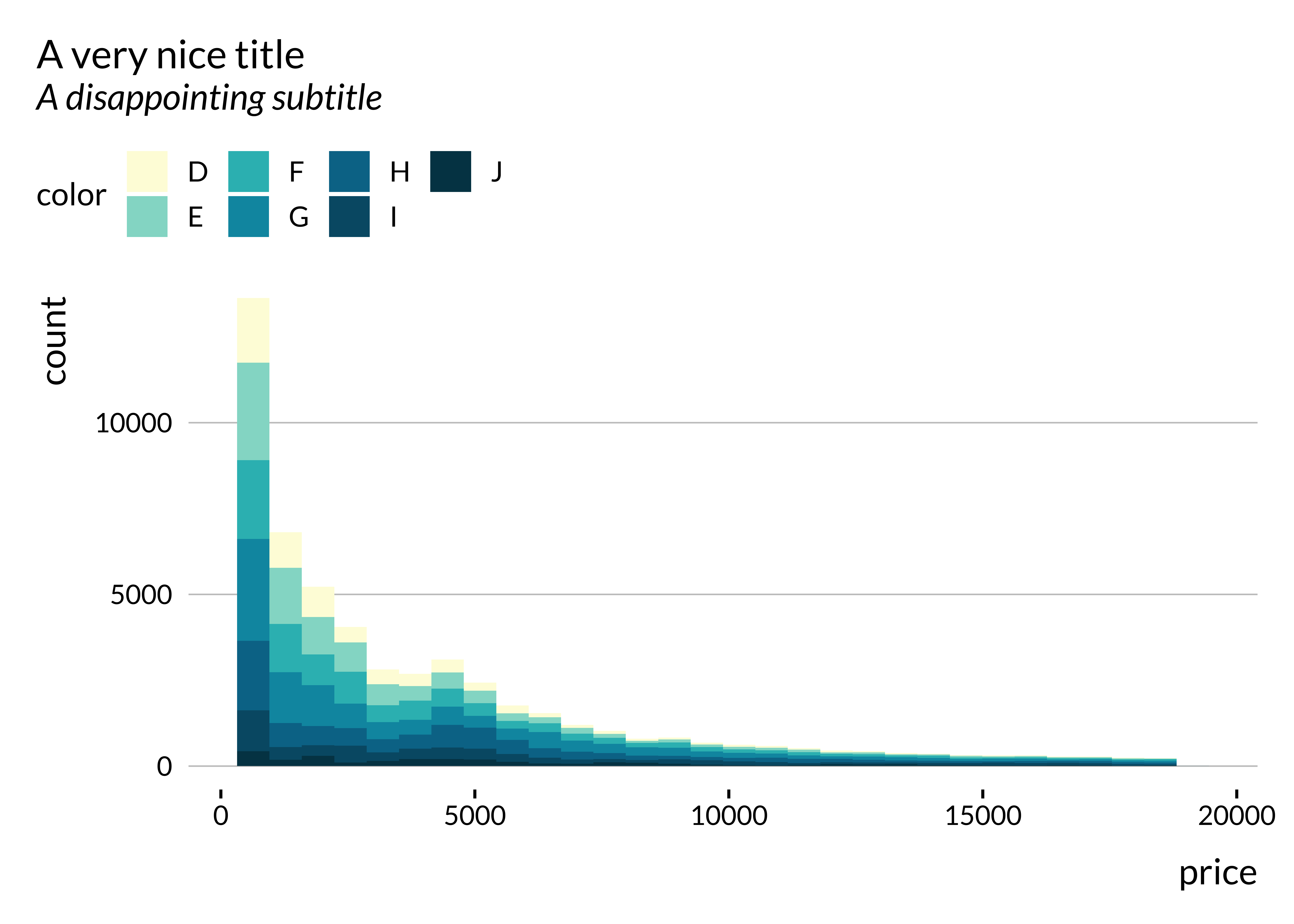
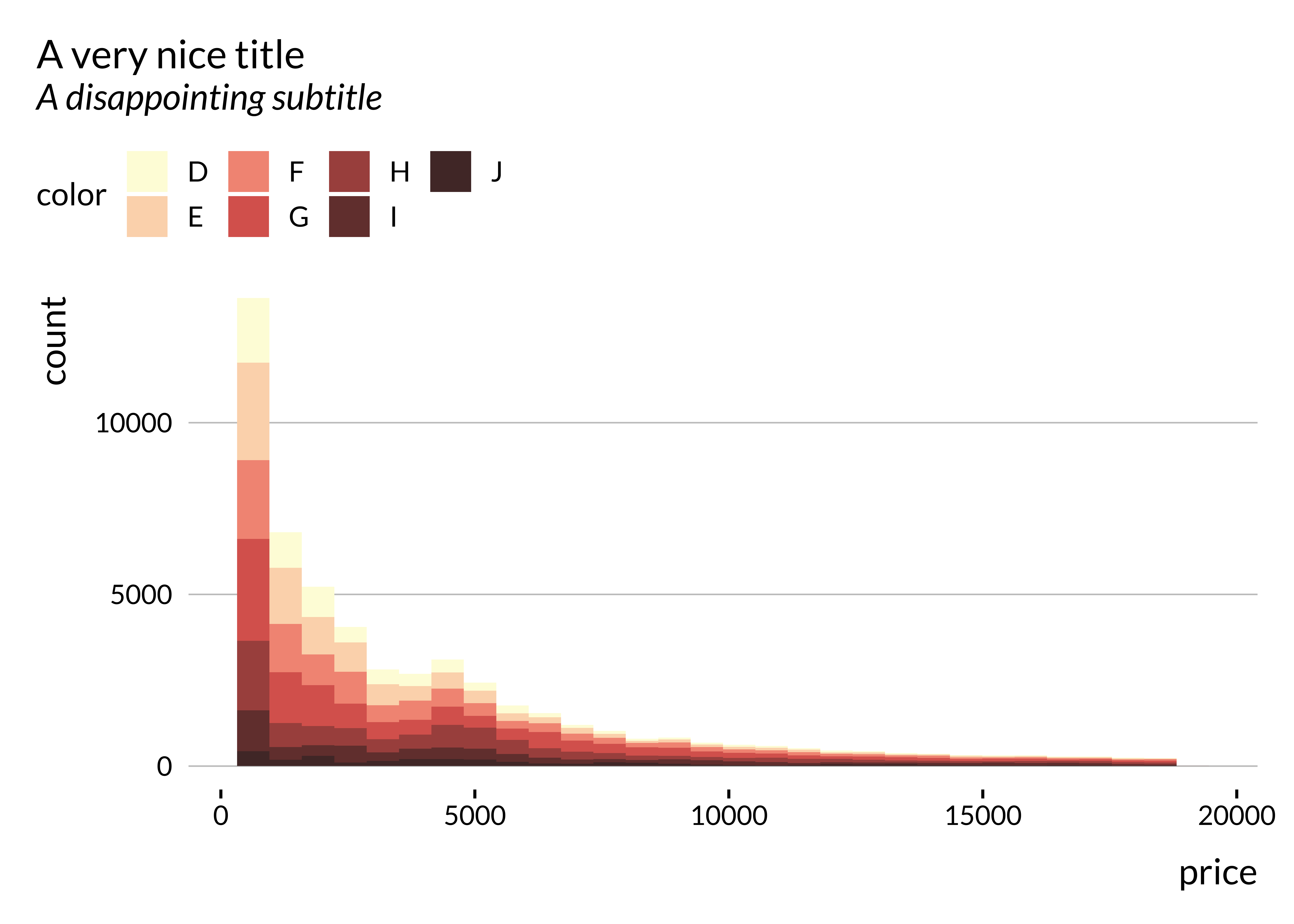
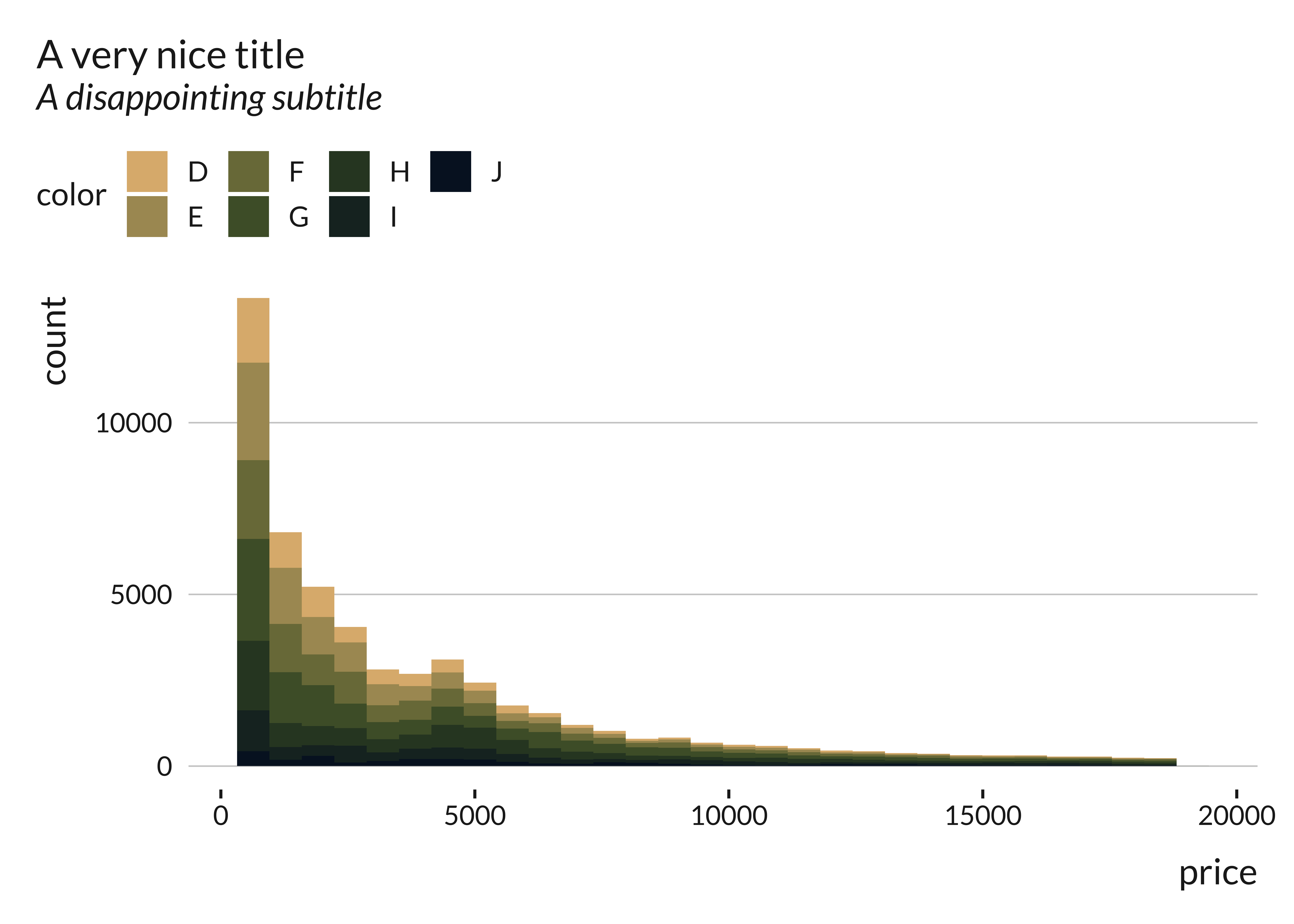
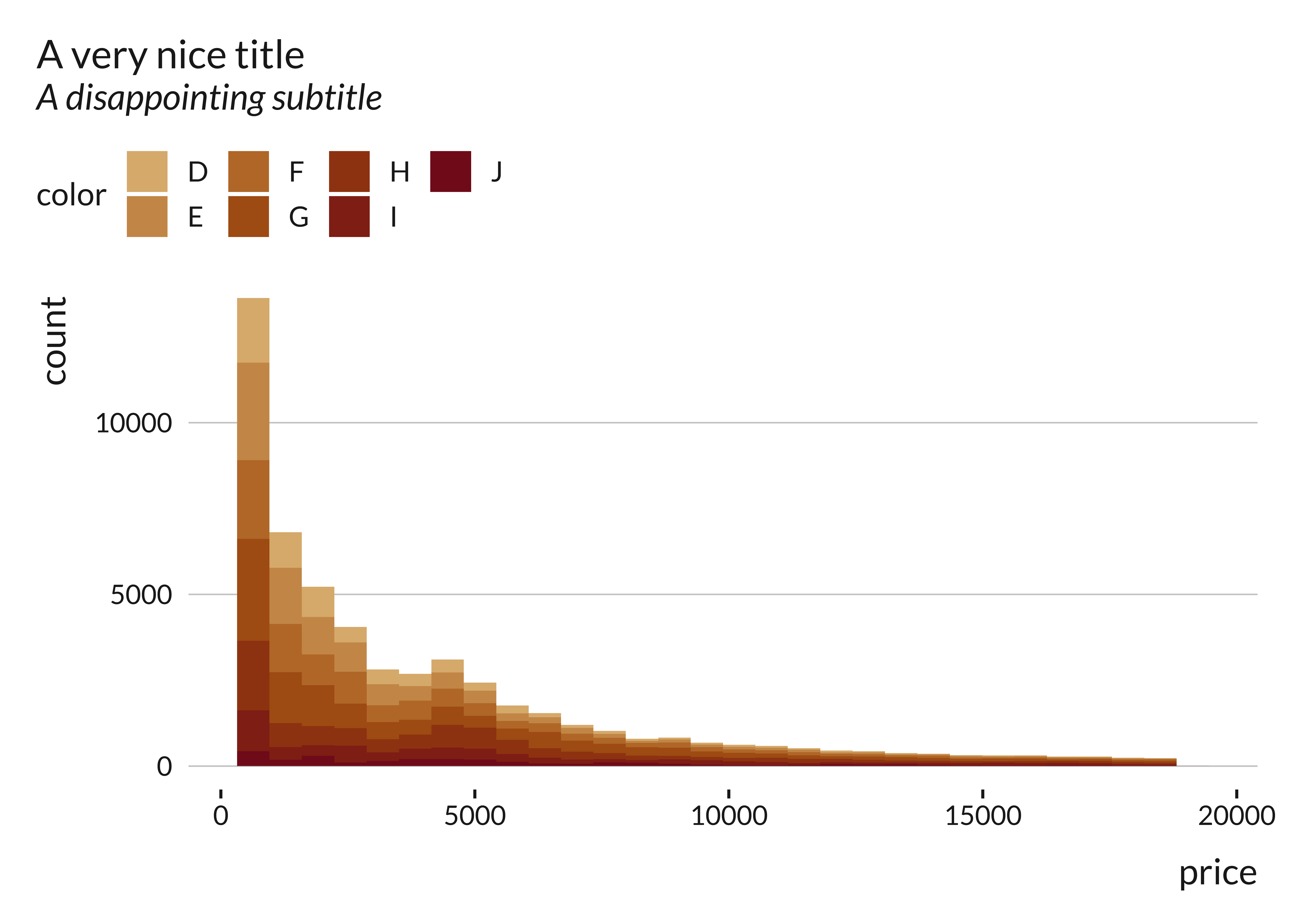
Each divergent palette (autumn, coty, rainbow and hotcold) can be
turned into two gradient palettes. This is done by splitting a divergent
palette in the middle, and use either the set of colors on the right or
on the left (flipped to get light colors for small values). The example
below hopefully clarifies this. To use these gradient palettes, one only
needs to set the parameter gradient to “left” or
“right”.
#> [1] "set_mediocre_all(pal = 'coty')"
#> `stat_bin2d()` using `bins = 30`. Pick better value `binwidth`.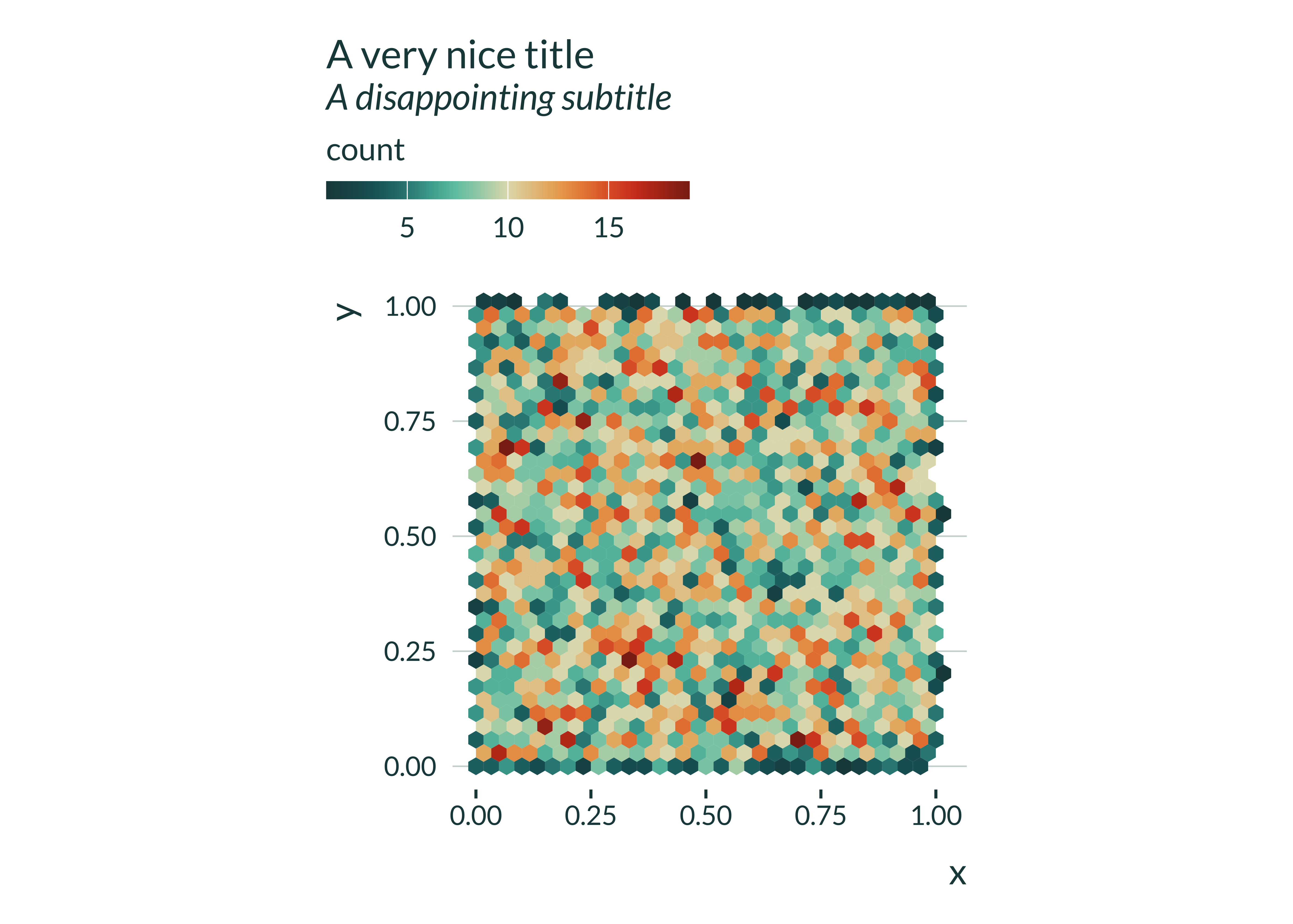
#> [1] "set_mediocre_all(pal = 'coty', gradient = 'left')"
#> `stat_bin2d()` using `bins = 30`. Pick better value `binwidth`.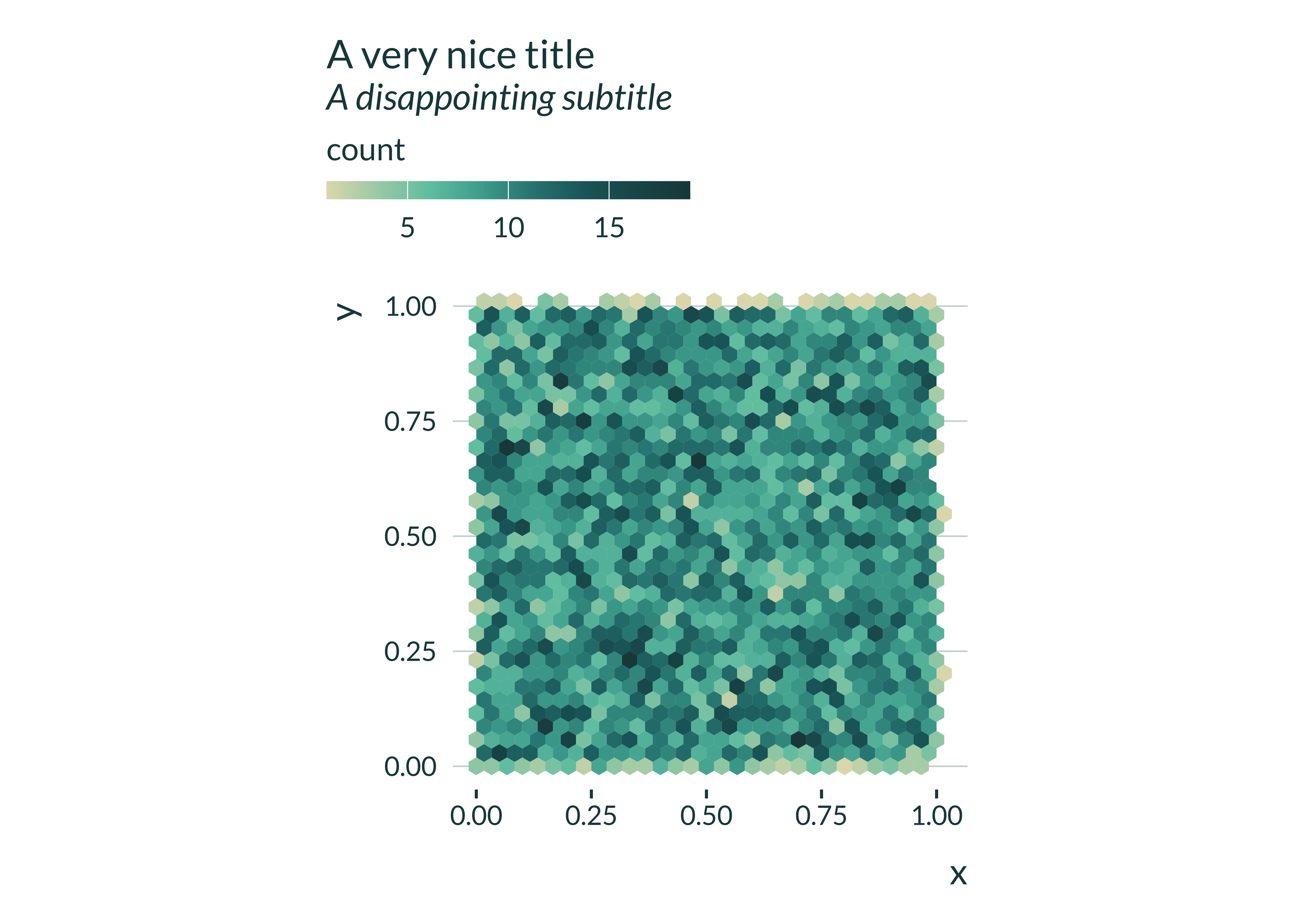
#> [1] "set_mediocre_all(pal = 'coty', gradient = 'right')"
#> `stat_bin2d()` using `bins = 30`. Pick better value `binwidth`.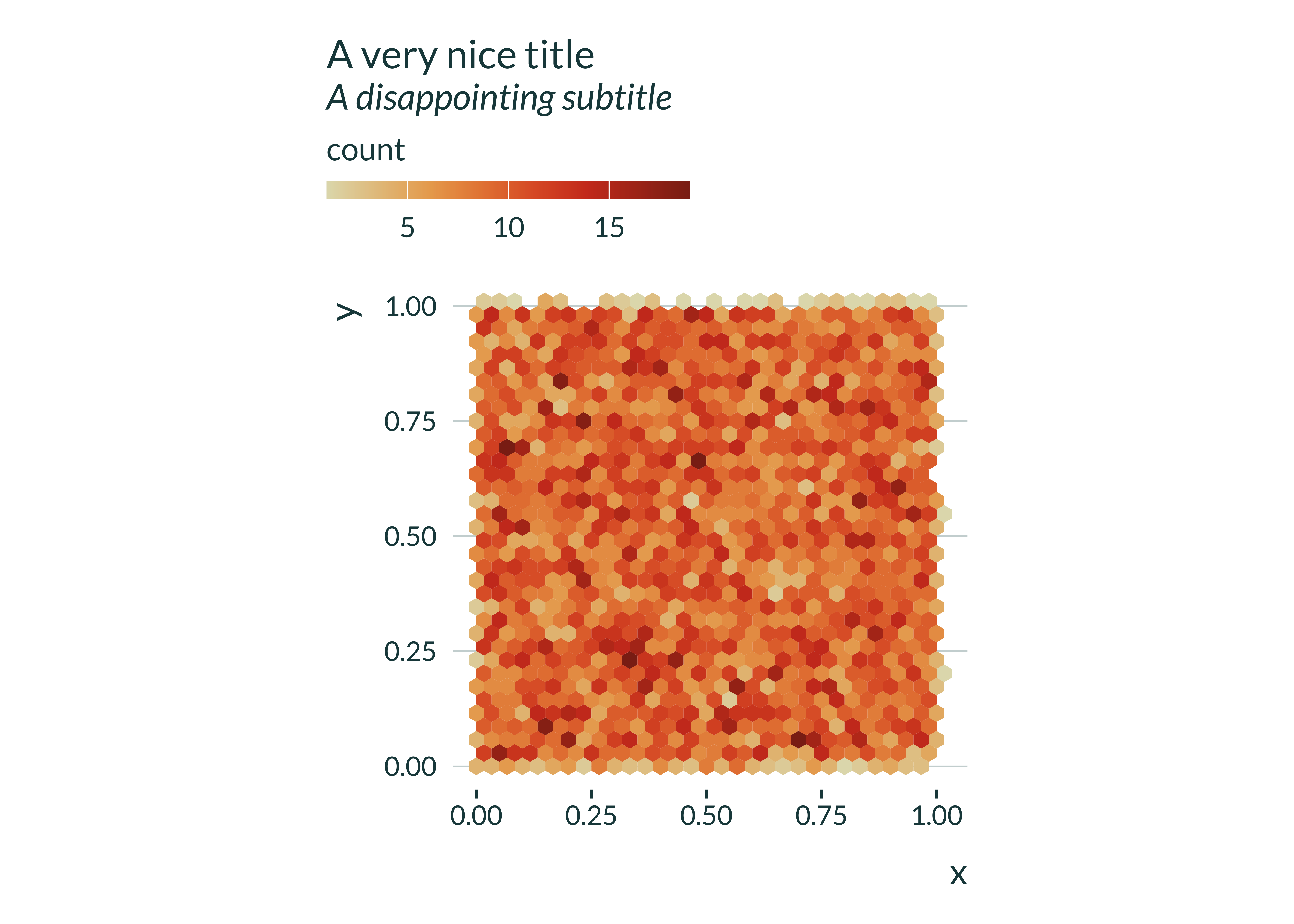
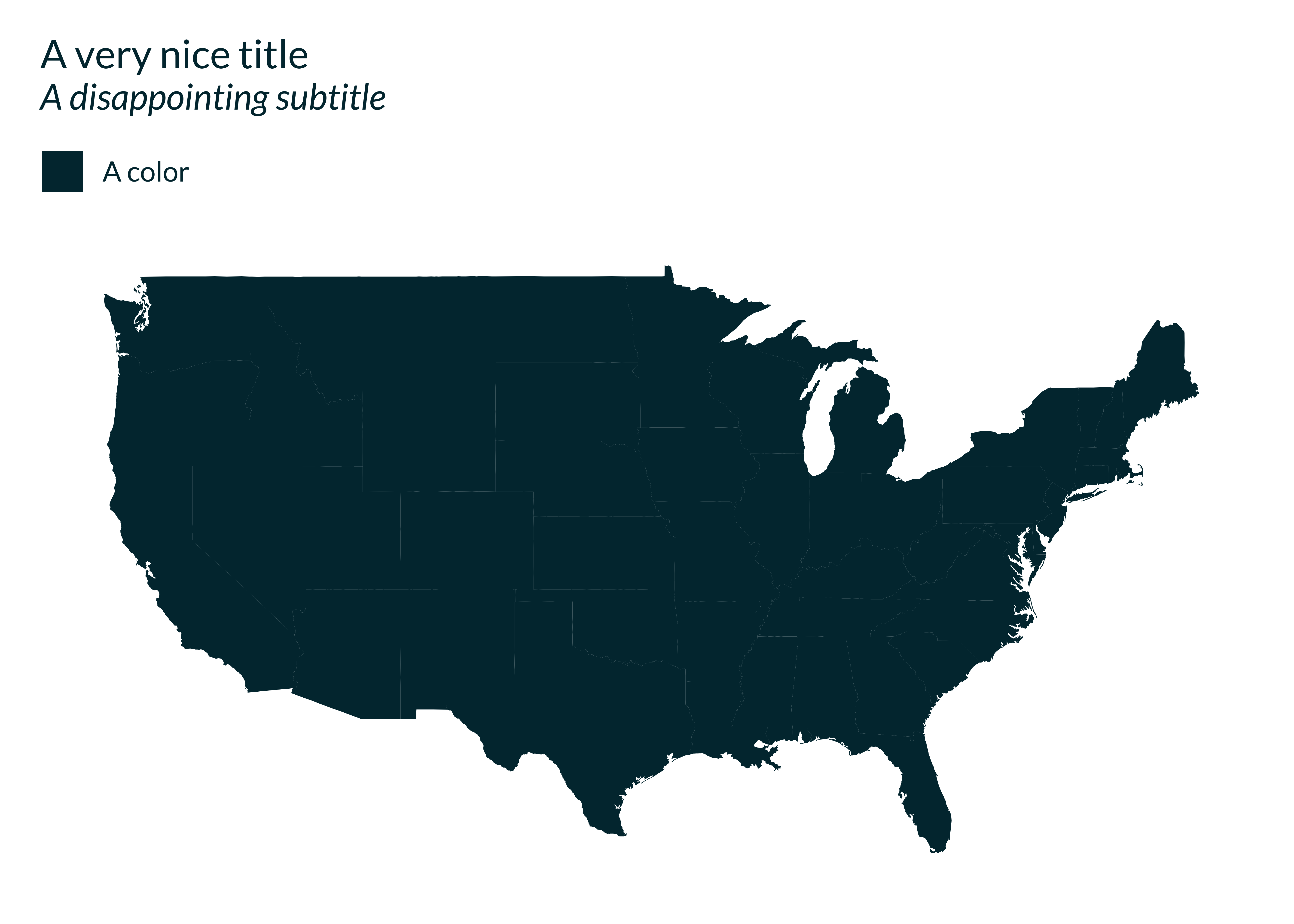
Theme for maps
When making maps, one can use the function
theme_mediocre_map() to apply a theme consistent with the
main (mediocre) one but without the unnecessary axis information (text,
ticks and panel grids).
One can remove the axis labels with the command
labs(x = NULL, y = NULL).
set_mediocre_all()

ggplot2::map_data("state") |>
  ggplot() +
  geom_polygon(aes(x=long, y=lat, group=group, fill = "A color")) +
  theme_mediocre_map() +
  coord_map(projection = "mercator") +
  labs(
    title = "A very nice title",
    subtitle = "A disappointing subtitle",
    fill = NULL,
    x = NULL, y = NULL
  )
Setting a background
Users can also easily set a background for all their plots by setting
the parameter background to TRUE. The color of
the background is predefined to fit nicely the theme palette. One can of
course still modify the background color by adding a layer to the ggplot
theme:
theme(plot.background = element_rect(fill = "red")).
set_mediocre_all(background = TRUE)

ggplot(data = ggplot2::mpg, aes(x = cty, y = displ)) +
    geom_point() +
    labs(title = "A very nice title", subtitle = "A disappointing subtitle")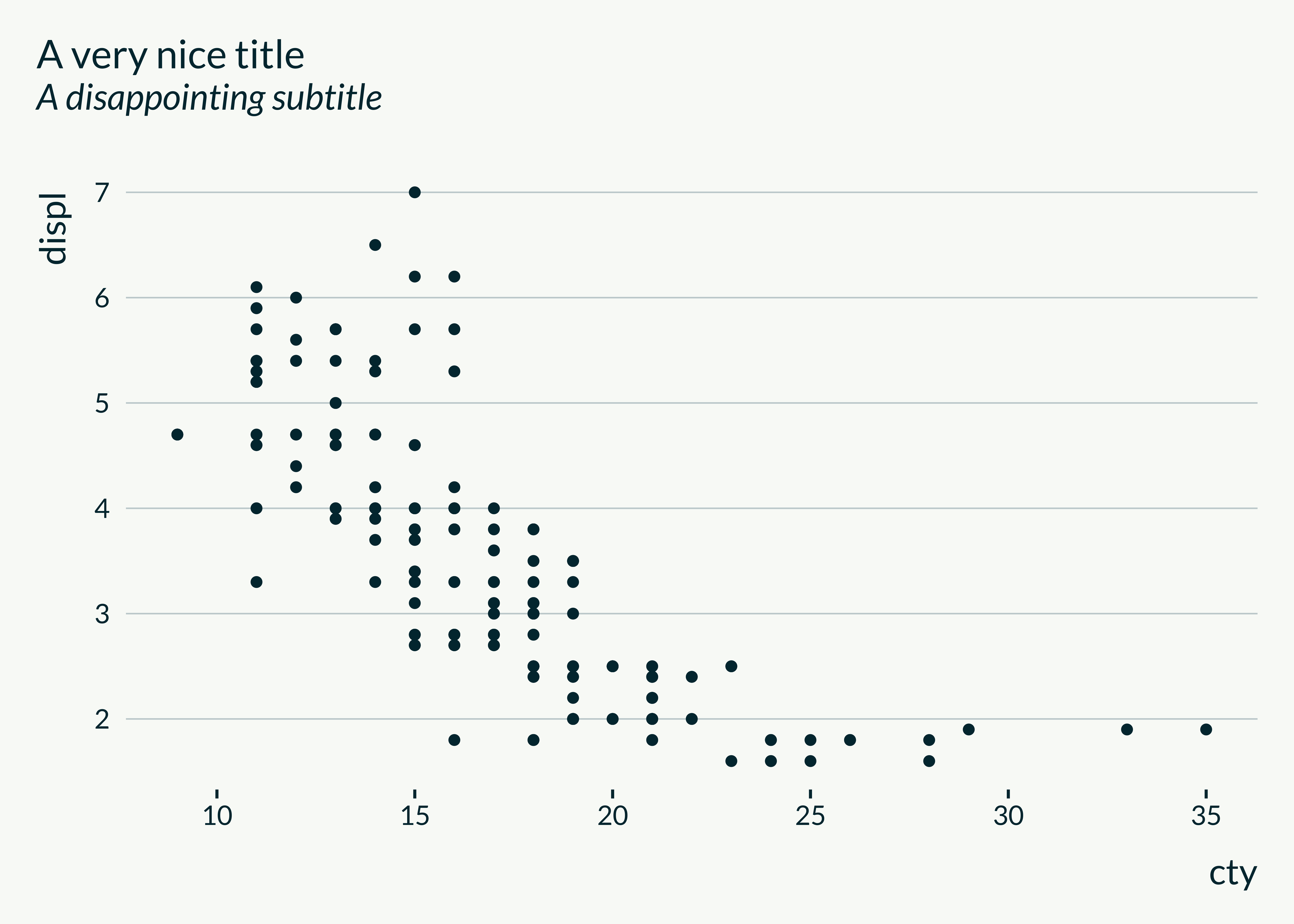
Using another pair of colors
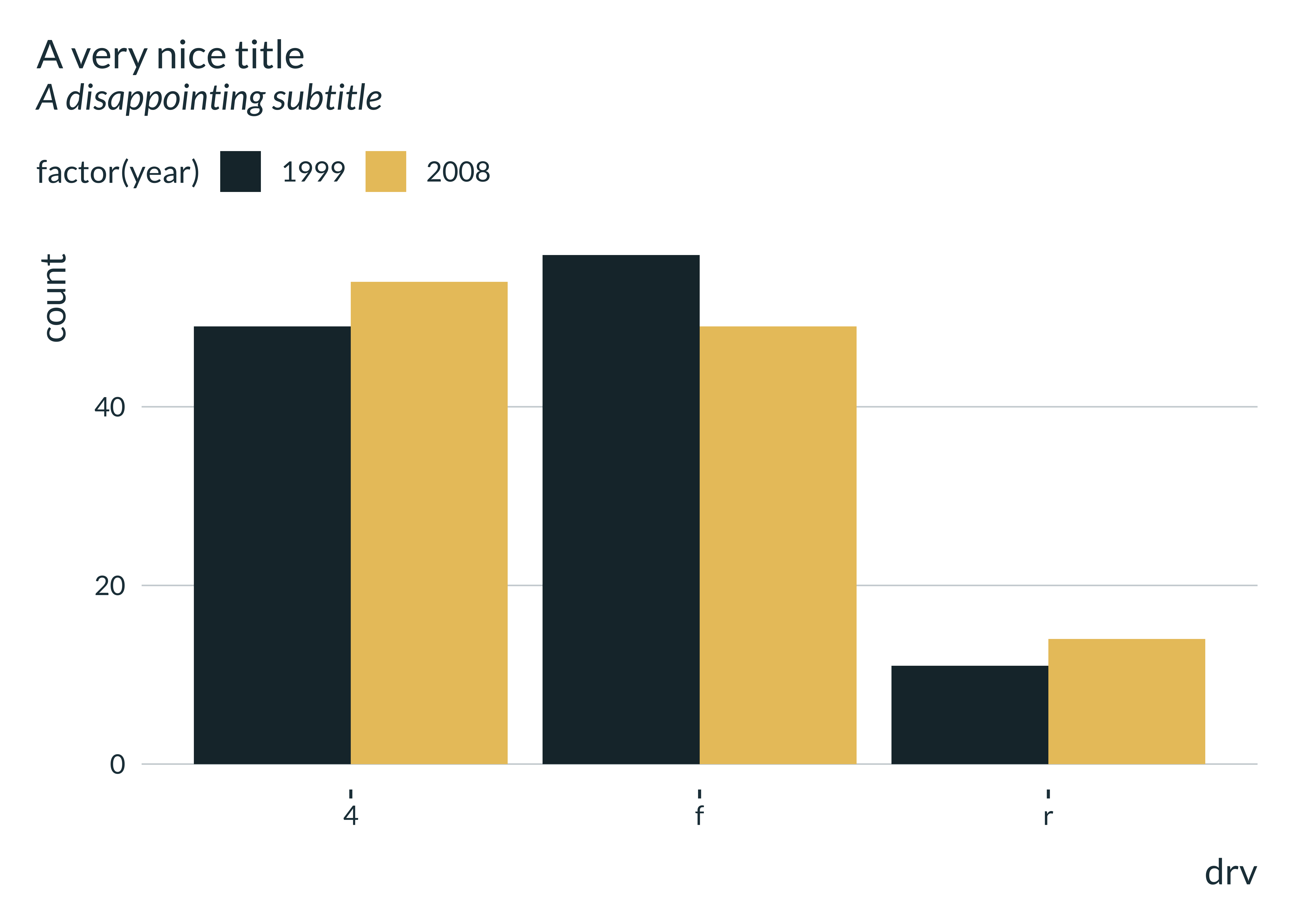
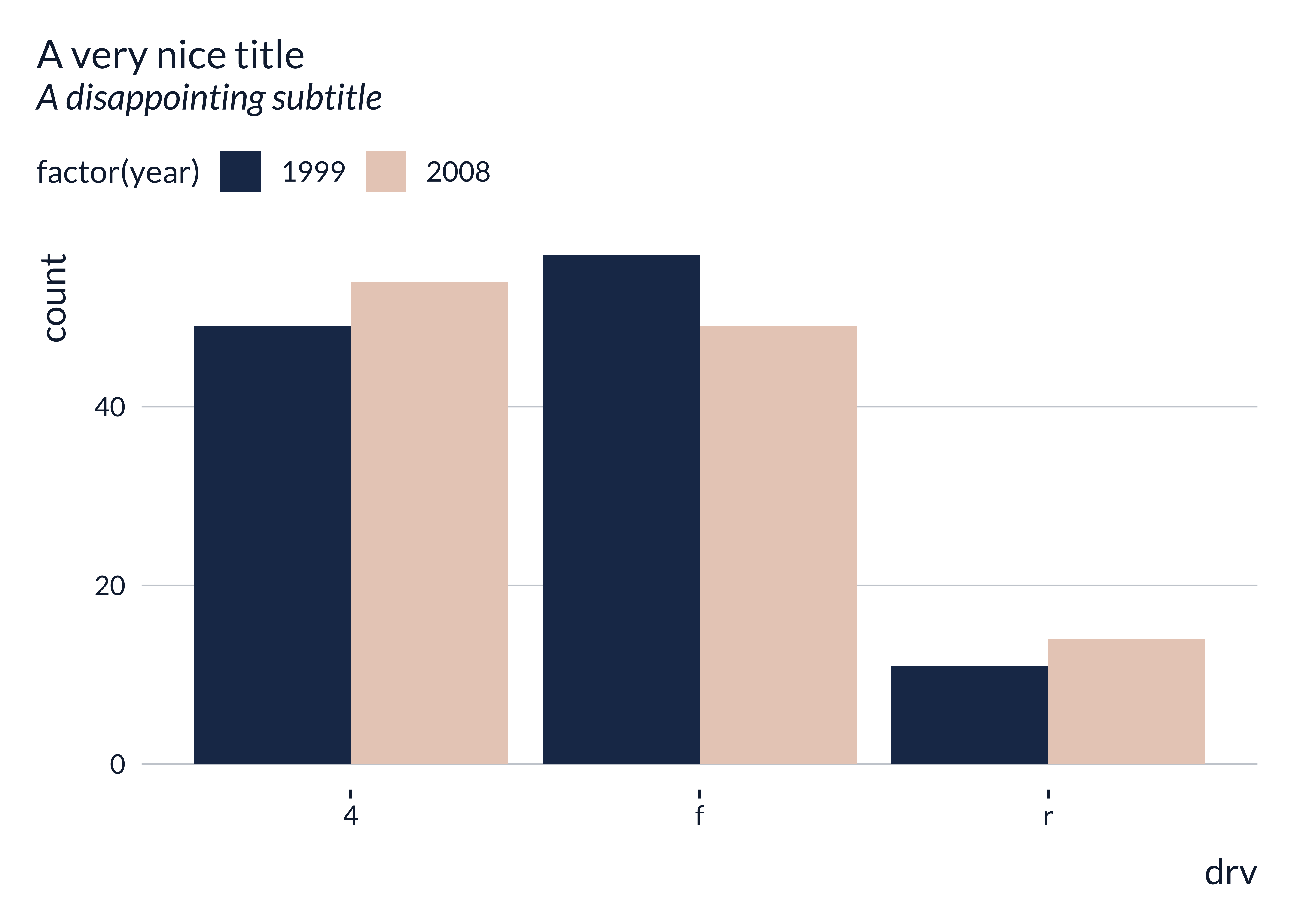
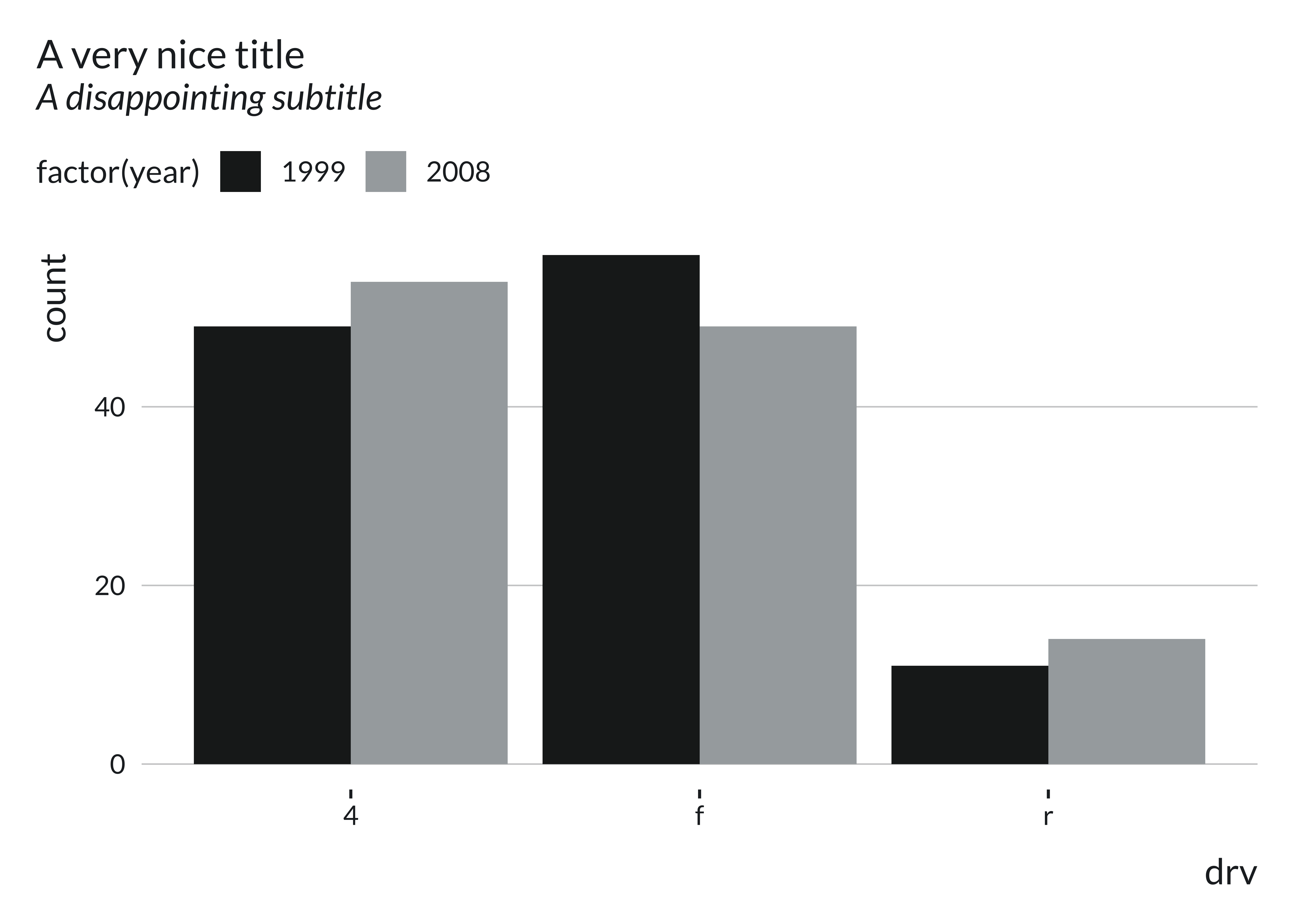
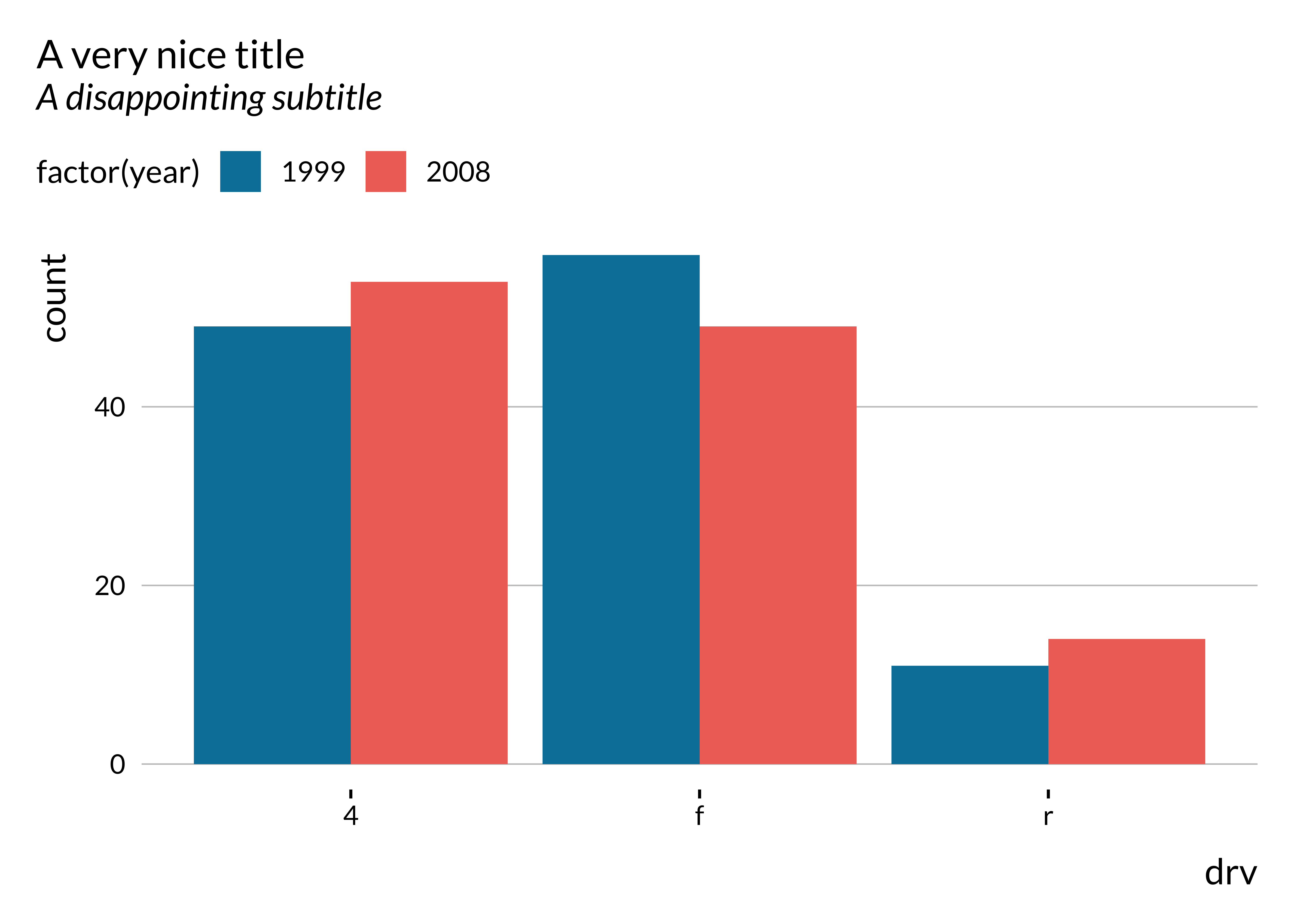
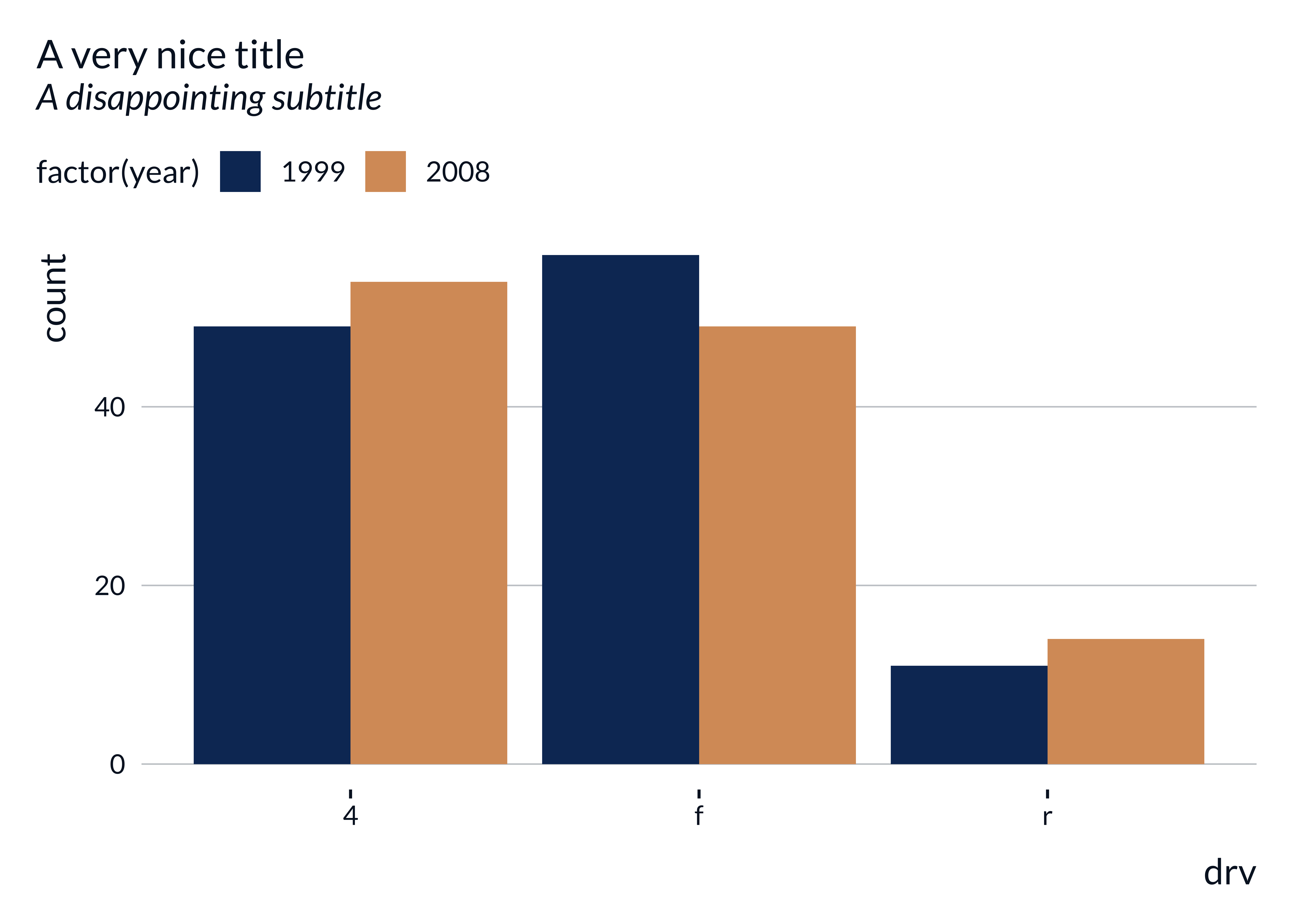
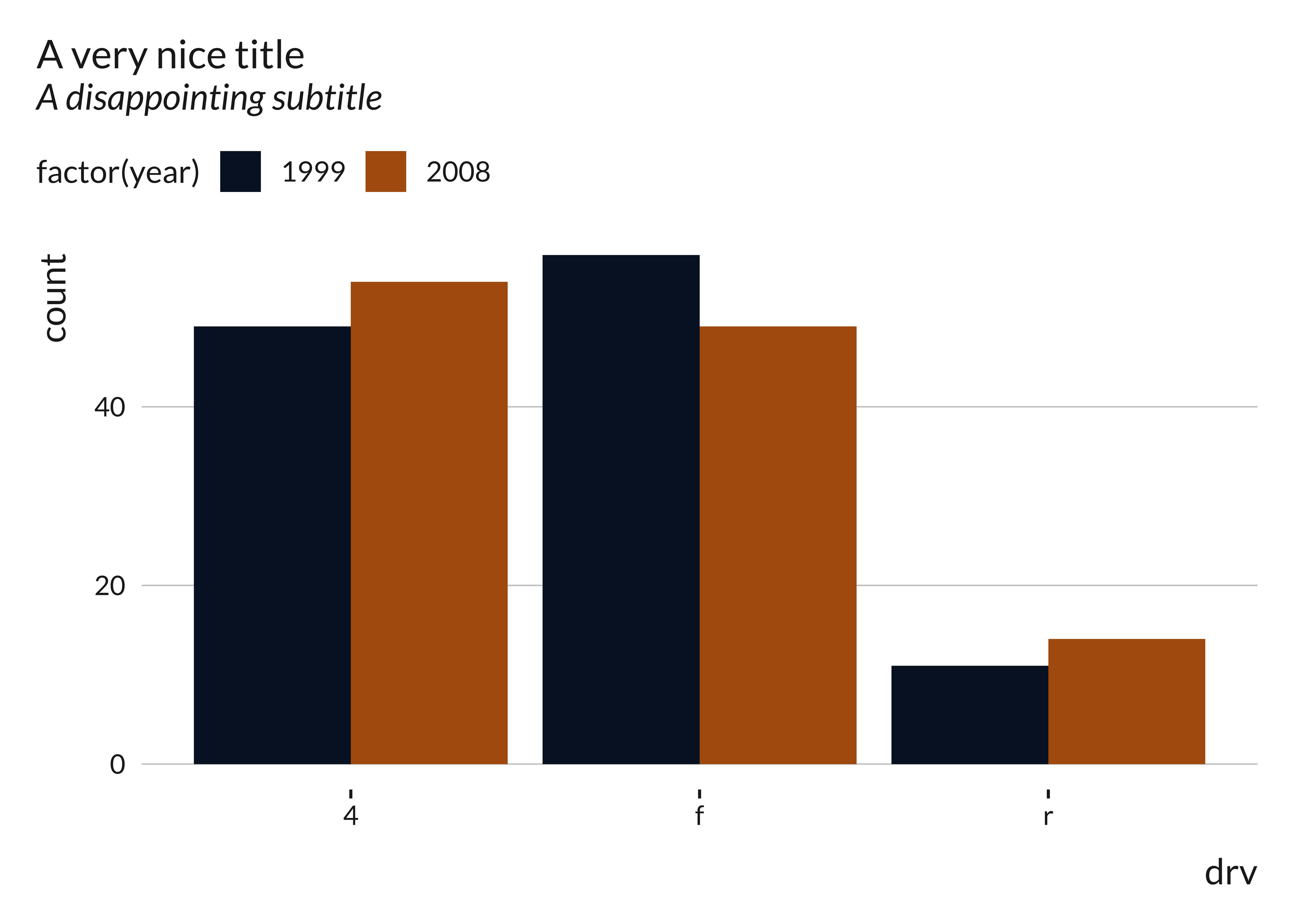
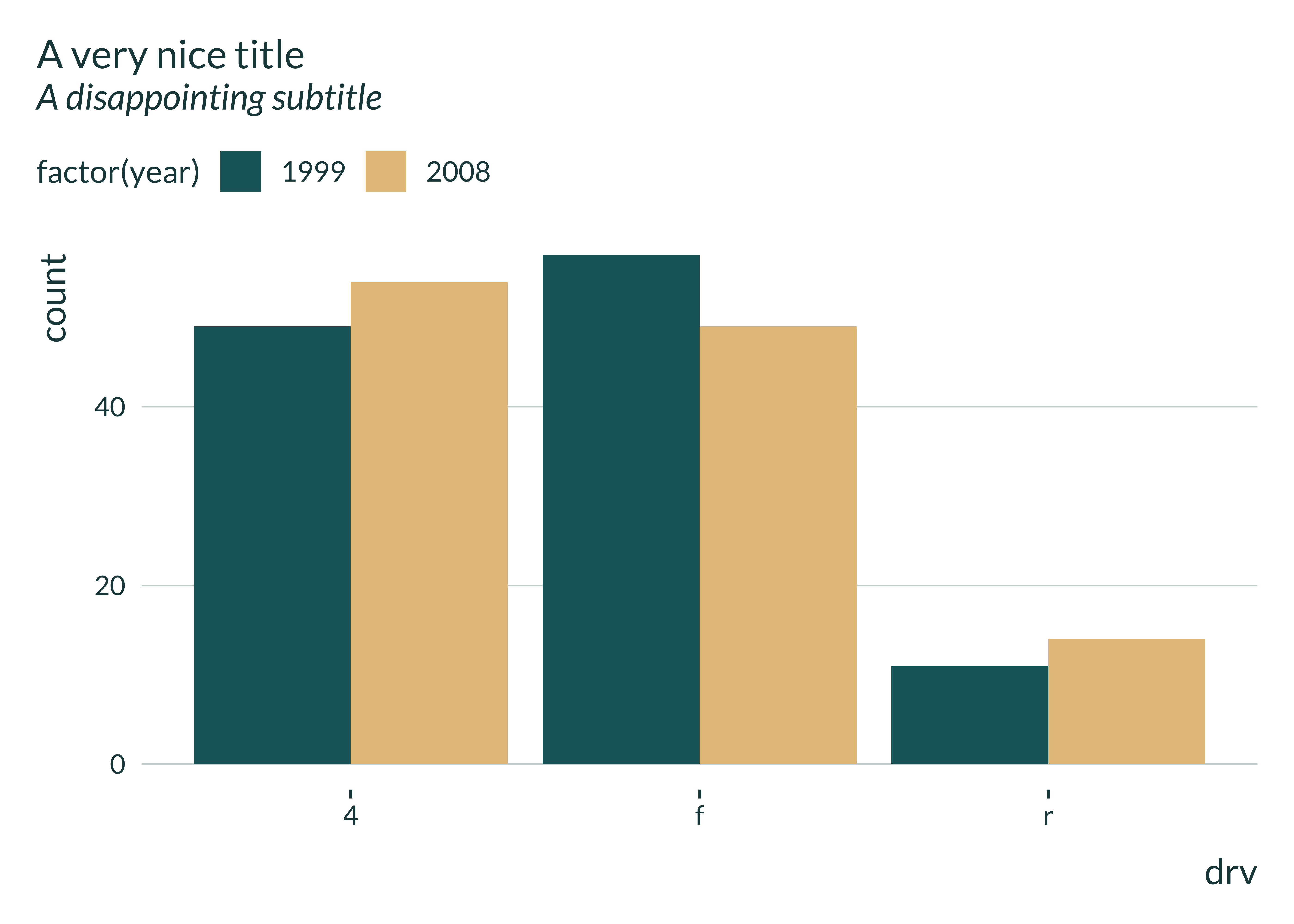
Graphs with two categories, as the following one for instance, are ubiquitous.
set_mediocre_all()

dat <- ggplot2::mpg |>
  dplyr::mutate(year = ifelse(drv == "f", NA, year))

ggplot(data = dat, aes(x = drv)) +
    geom_bar(aes(fill = factor(year)), position = "dodge") +
    labs(title = "A very nice title", subtitle = "A disappointing subtitle")
In a same project, users may have to consider different sets of
pairs. For instance, they may want to separate observations in years as
in the previous graph and later use other categories such as Republicans
and Democrats. User may not want to use the same color pair to denote
year and party. For instance they may not want Republicans to be coded
with the same color as the year 1999. To access a second color pair,
users can therefore set the second_pair parameter of
set_mediocre_all to TRUE and keep on writing
standard ggplot code. Subsequent bi-color graphs will use a second pair
of colors, different from the base one but still consistent with the
color scale used.
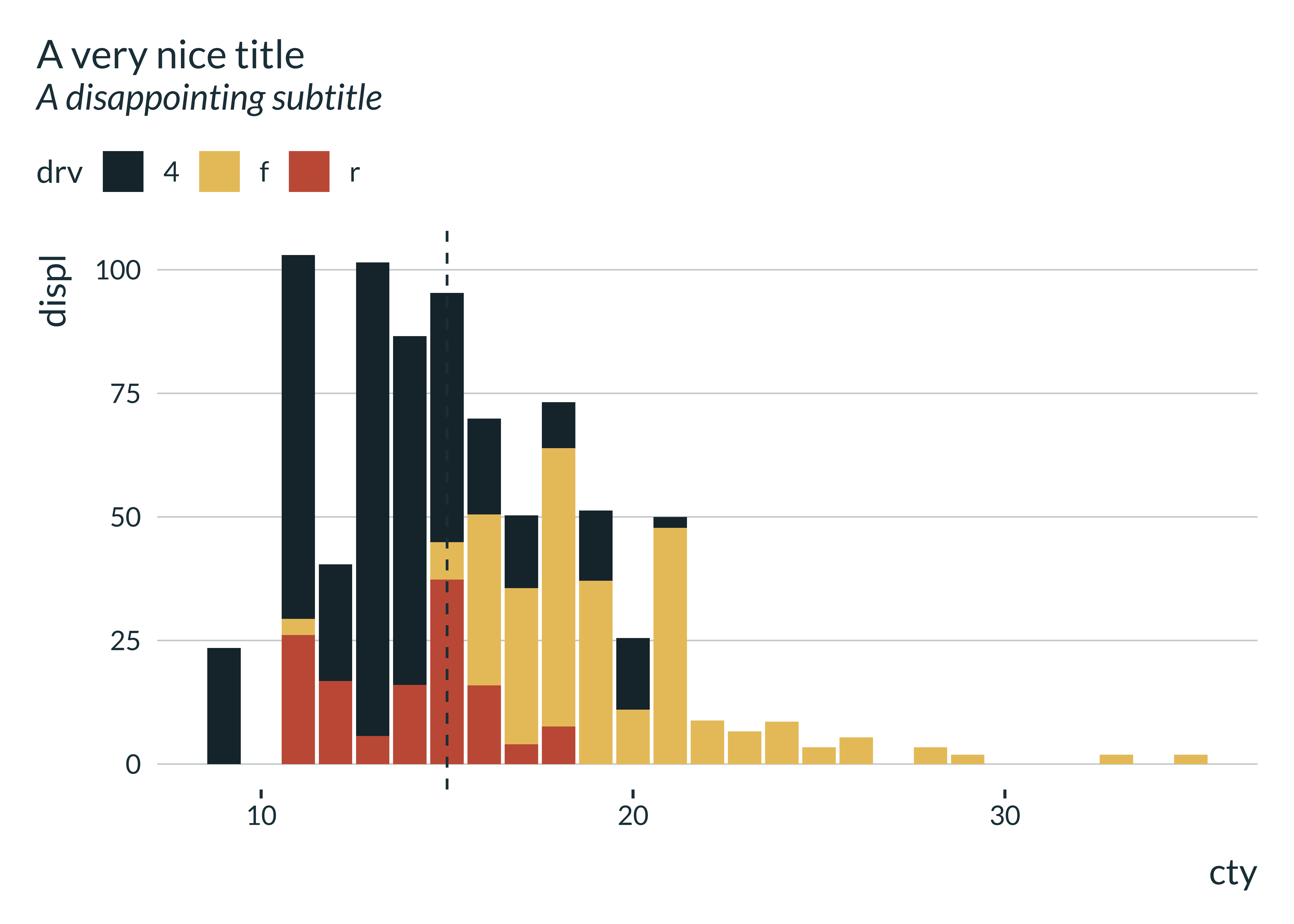
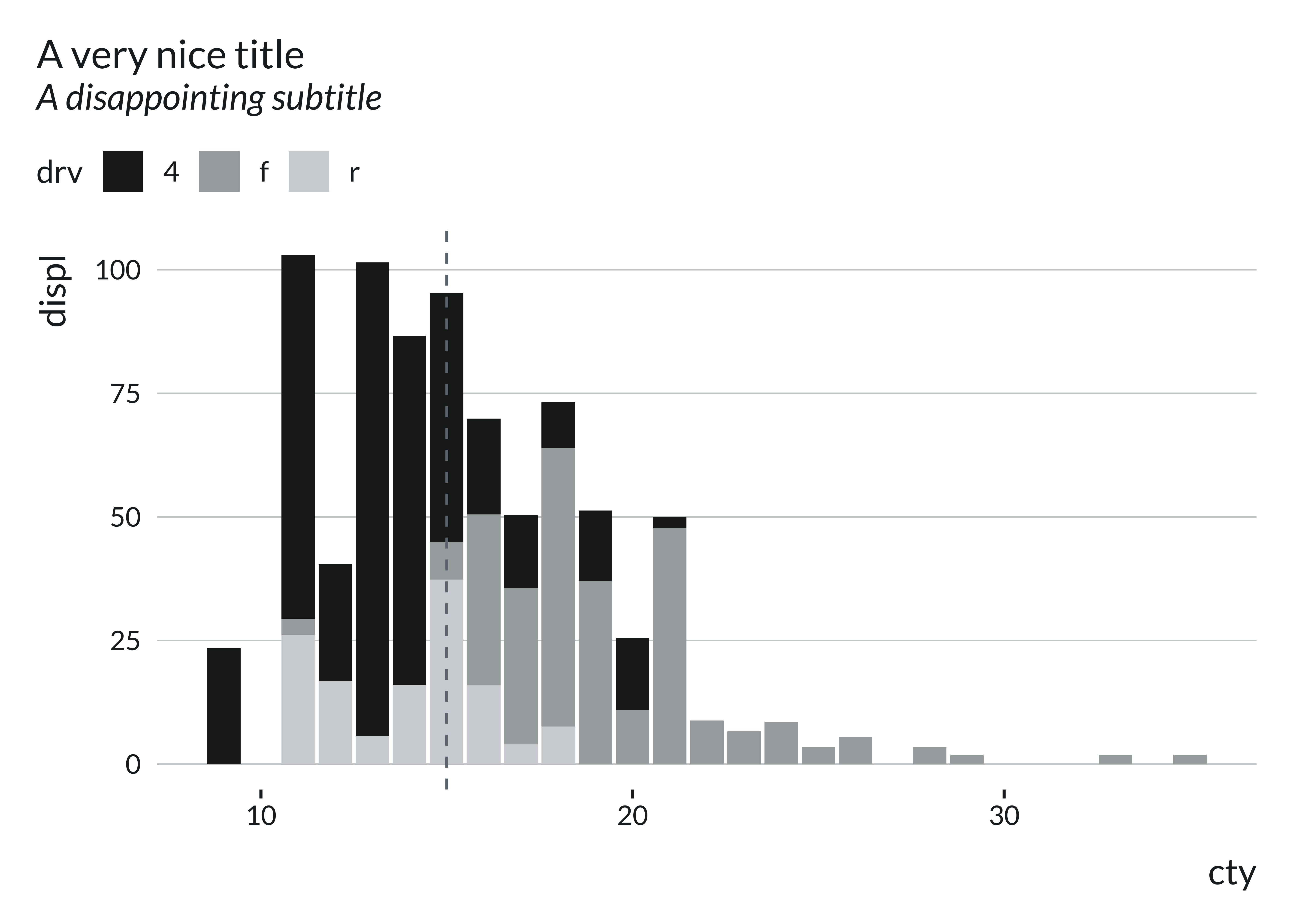
set_mediocre_all(second_pair = TRUE)

ggplot(data = ggplot2::presidential, aes(x = party)) +
  geom_bar(aes(fill = party), position = "dodge") +
  labs(title = "A very nice title", subtitle = "A disappointing subtitle")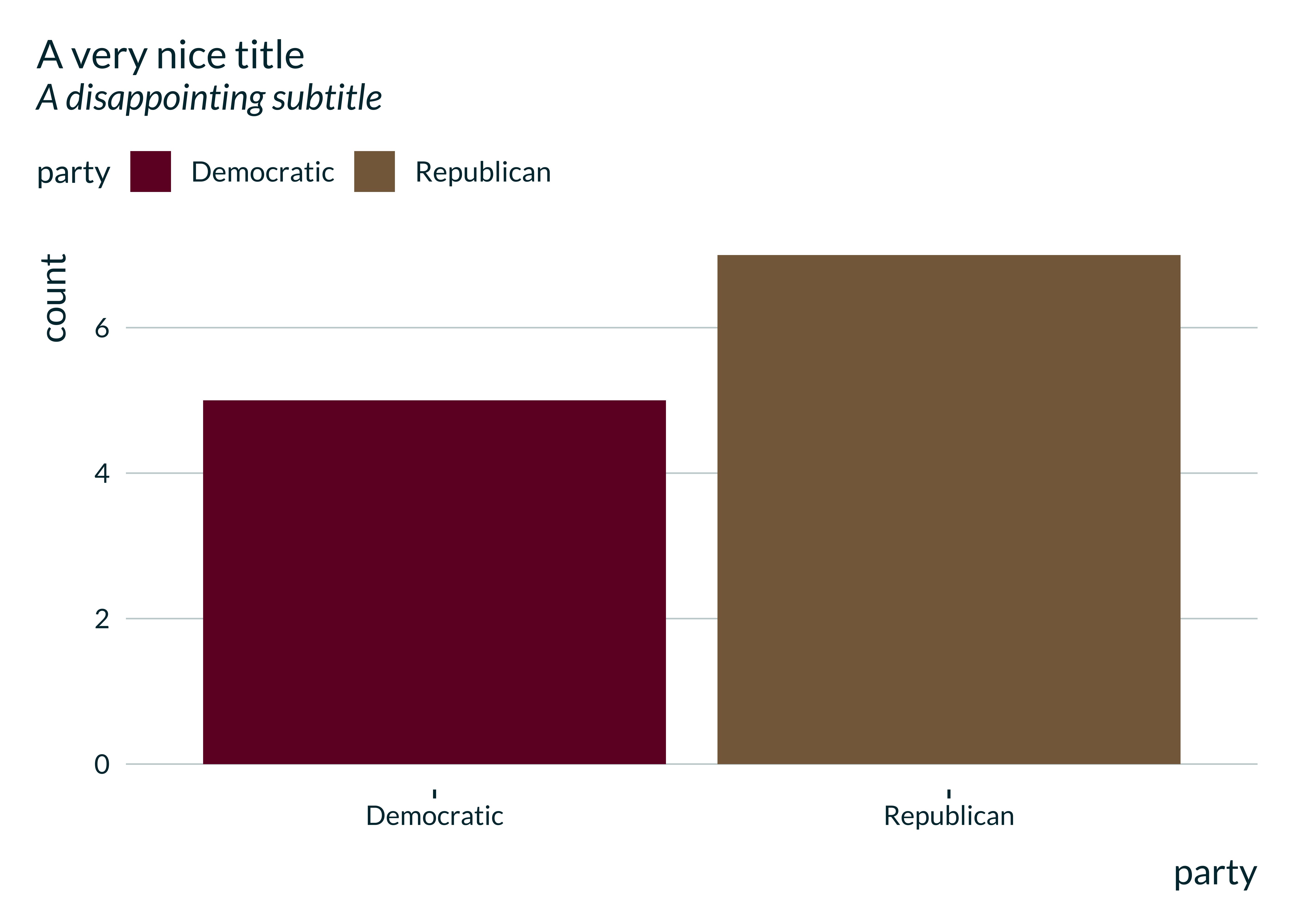
Accessing the colors in the current palette
As a side effect, the function set_mediocre_all returns
a one line tibble (colors_mediocre) with all the color
information relative to the current palette:
| pal | base | text | background | complementary | vector | four_colors |
|---|---|---|---|---|---|---|
| autumn | #00313C | #00313C | #F9FAF7 | #FB9637 | #00313C, #183C41, #304746, #48514A, #856949, #AB7743, #D2863C, #FB9637, #E57630, #D0562B, #BC3626, #A61922, #8D0422, #70002A, #520036 | #00313C, #FB9637, #856949, #70002A |
Thus, to access the base color for instance, one should use the following command:
colors_mediocre[["base"]]
#> [1] "#00313C"